Ch07 Symmetric Matrices and Quadratic Forms

7.2 Quadratic Forms

A quadratic form on $\mathbb{R}^n$ is a function $Q$ defined on $\mathbb{R}^n$ whose value at a vector $\textbf{x}$ in $\mathbb{R}^n$ can be computed by an expression of the form $Q(\textbf{x}) = \textbf{x}^T A \textbf{x}$, where $A$ is an $n \times n$ symmetric matrix. The matrix $A$ is called the matrix of the quadratic form.

The simplest example of a nonzero quadratic form is $Q(\textbf{x}) = \textbf{x}^T I \textbf{x} = ||\textbf{x}||^2$. Examples 1 and 2 show the connection between any symmetric matrix $A$ and the quadratic form $\textbf{x}^T A \textbf{x}$.

Example 1

Let $\textbf{x}=\begin{bmatrix} x_1 \\ x_2 \end{bmatrix}$. Compute $\textbf{x}^TA\textbf{x}$ for the following matrices:

a. $A=\begin{bmatrix} 4 & 0 \\ 0 & 3 \end{bmatrix}$

b. $A=\begin{bmatrix} 3 & -2 \\ -2 & 7 \end{bmatrix}$

Solution

omit

$\blacksquare$

The presence of $-4x_1x_2$ in the quadratic form in Example 1(b) is due to -2 entries off the diagonal in the matrix $A$. In contrast, the quadratic form associated with the diagonal matrix $A$ in Example 1(a) has no $x_1 x_2$ cross-product term.

Example 2

For $\textbf{x} \in \mathbb{R}^3$, let $Q(\textbf{x})=5x_1^2+3x_2^2+2x_3^2-x_1x_2+8x_2x_3$. Write this quadratic form as $x^TAx$.

Solution

The coefficients of $x_1^2, x_2^2, x_3^2$ go on the diagonal of $A$. To make $A$ symmetric, the coefficient of $x_ix_j$ for $i \ne j$ must be split evenly between the $(i,j)$-and $(j,i)$-entries in $A$. The coefficients of $x_1x_3$ is 0. It is readily checked that

$$Q(\textbf{x}) = \textbf{x}^T A \textbf{x} = \begin{bmatrix} x_1 & x_2 & x_3 \end{bmatrix} \begin{bmatrix} 5 & -1/2 & 0 \\ -1/2 & 3 & 4 \\ 0 & 4 & 2 \end{bmatrix} \begin{bmatrix} x_1 \\ x_2 \\ x_3 \end{bmatrix} \blacksquare$$

Change Variable in a Quadratic Form

If $\textbf{x}$ represents a variable vector in $\mathbb{R}^n$ , then a change of variable is an equation of the form

$$\textbf{x} = P\textbf{y}, \text{ or equivalently, }\textbf{y} = P^{-1}\textbf{x} \tag{1}$$

where $P$ is an invertible matrix and $\textbf{y}$ is a new variable vector in $\mathbb{R}^n$.

Here $\textbf{y}$ is the coordinate vector of $\textbf{x}$ relative to the basis of $\mathbb{R}^n$ determined by the columns of $P$. (See Section 4.4.)

If the change of variable (1) is made in a quadratic form $\textbf{x}^TA\textbf{x}$, then

$$\textbf{x}^TA\textbf{x} = (P\textbf{y})^TA(P\textbf{y}) = \textbf{y}^TP^TAP\textbf{y} = \textbf{y}^T(P^TAP)\textbf{y} \tag{2}$$

and the new matrix of the quadratic form is $P^T AP$.

Since $A$ is symmetric, Theorem 2 guarantees that there is an orthogonal matrix $P$ such that $P^T AP$ is a diagonal matrix $D$,and the quadratic form in (2) becomes $\textbf{y}^T D\textbf{y}$.

Example 4

Make a change of variable that transforms the quadratic form $Q(\textbf{x})=x_1^2-8x_1x_2-5x_2^2$ into a quadratic form with no cross-product term.

Solution of Example 4

The matrix of the given quadratic form is

$$A = \begin{bmatrix} 1 & -4 \\ -4 & -5 \end{bmatrix}$$

The first step is to orthogonally diagonalize $A$ Its eigenvalues turn out to be $\lambda=3$ and $\lambda=-7$. Associated unit eigenvectors are

$$\lambda=3: \begin{bmatrix} 2/\sqrt{5} \\ -1/\sqrt{5} \end{bmatrix}; \lambda=-7: \begin{bmatrix} 1/\sqrt{5} \\ 2/\sqrt{5} \end{bmatrix}$$

These vectors are automatically orthogonal (because they correspond to distinct eigenvalues) and so provide an orthonormal basis for $\mathbb{R}^n$. Let $$P= \begin{bmatrix} 2/\sqrt{5} & 1/\sqrt{5} \\ -1/\sqrt{5} & 2/\sqrt{5} \end{bmatrix}, D= \begin{bmatrix} 3 & 0 \\ 0 & -7 \end{bmatrix}$$

Then $A=PDP^{-1}$ and $D=P^{-1}AP=P^T AP$.

A suitable change of variable is

$$\textbf{x}=P\textbf{y}, \text{ where } \textbf{x}=\begin{bmatrix} x_1 \\ x_2\end{bmatrix} \text{ and } \textbf{y}=\begin{bmatrix} y_1 \\ y_2\end{bmatrix}$$

Then

$$\begin{align*} x_1^2-8x_1x_2-5x_2^2 &= \textbf{x}^TA\textbf{x} = (P\textbf{y})^TA(P\textbf{y}) \\ &= \textbf{y}^TP^T A P\textbf{y} = \textbf{y}^T D \textbf{y} \\ &= 3y_1^2-7y_2^2 \end{align*} \blacksquare$$

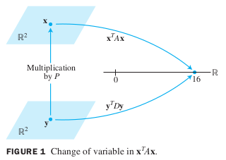
To illustrate the meaning of the equality of quadraticforms in Example 4, we can compute $Q(\textbf{x})$ for $\textbf{x}=(2,-2)$ using the new quadratic form.

First, since $\textbf{x}=P\textbf{y}$,

$$\textbf{y}=P^{-1}\textbf{x}=P^T\textbf{x}$$

so

$$\textbf{y}= \begin{bmatrix} 2/\sqrt{5} & -11/\sqrt{5} \\ 1/\sqrt{5} & 2/\sqrt{5} \end{bmatrix} \begin{bmatrix} 2 \\ -2 \end{bmatrix} = \begin{bmatrix} 6/\sqrt{5}\\ -2/\sqrt{5} \end{bmatrix}$$

Hence

$$\begin{align*} 3y_1^2-7y_2^2 &= 3(\frac{6}{\sqrt{5}})^2 - 7(\frac{-2}{\sqrt{5}})^2 \\ &=3\frac{36}{5}-7\frac{4}{5} \\ &=\frac{80}{5} \\ &=16 \end{align*}$$

This is the value of $Q(\textbf{x})$ when $\textbf{x}=(2,-2)$.

See the fiqure below.

Theorem 4

The Pricipal Axes Theorem

Let $A$ be an symmetric matrix. Then there is an orthogonal change of variable, $\textbf{x}=P\textbf{y}$ that transforms the quadratic form $\textbf{x}^T A\textbf{x}$ into a quadratic form $\textbf{y}^TD\textbf{y}$ with no cross-product term.

The columns of $P$ in Theorem 4 are called the principal axes of the quadratic form $\textbf{x}^TA\textbf{x}$.

The vector $\textbf{y}$ is the coordinate vector of $\textbf{x}$ relative to the orthonormal basis of $\mathbb{R}^n$ given by these principle axes.

A Geometric View of Pricipal Axes

Suppose $Q(\textbf{x})=\textbf{x}^TA\textbf{x}$, where $A$ is an invertible $2 \times 2$ symmetric matrix, and let $c$ be a constant.

It can be shown that the set of all $\textbf{x}$ in $\mathbb{R}^2$ that satisfy

$$\textbf{x}^TA\textbf{x}=c \tag{3}$$

either corresponds to an ellipse (or circle), a hyperbola, two intersecting lines, or a single point, or contains no points at all.

If $A$ is a diagonal matrix, the graph is in standard position, such as in the figure below.

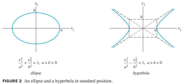
If $A$ is not a diagonal matrix, the graph of equation (3) is rotated out of standard position, as in the figure below.

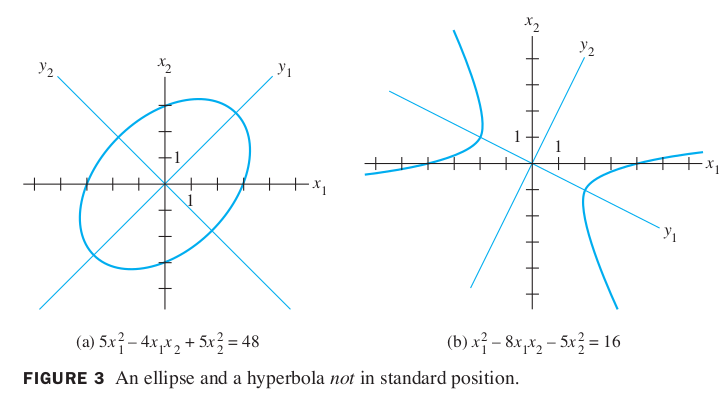
Finding the principal axes (determined by the eigenvectors of $A$) amounts to finding a new coordinate system with respect to which the graph is in standard position.

Classifying Quadratic Forms

A quadratic form Q is:

1. positive definite if $Q(\textbf{x}) > 0$ for all $\textbf{x} \ne 0$
2. negative definite if $Q(\textbf{x}) < 0$ for all $\textbf{x} \ne 0$
3. indefinite if $Q(\textbf{x})$ assumes both positive and negative values.

Also, $Q$ is said to be positive semidefinite if $Q(\textbf{x}) \ge 0$ for all $\textbf{x}$, and negative semidefinite if $Q(\textbf{x}) \le 0$ for all $\textbf{x}$.

Quadratic Forms and Eigenvalues

Theorem 5

Let $A$ be an $n \times n$ symmetric matrix. Then a quadratic form $\textbf{x}^TA\textbf{x}$ is:

1. positive definite if and only if the eigenvalues of $A$ are all positive,
2. negative definite if and only if the eigenvalues of $A$ are all negative, or
3. indefinite if and only if $A$ has both positive and negative eigenvalues.

Proof

By the Principal Axes Theorem, there exists an orthogonal change of variable $\textbf{x}=P\textbf{y}$ such that

$$Q(\textbf{x}) = \textbf{x}^T A \textbf{x} = \textbf{y}^T D \textbf{y} = \lambda_1y_1^2 + \lambda_2y_2^2 + \cdots + \lambda_ny_n^2 \tag{4}$$ where $\lambda_1, \cdots \lambda_n$ are the eigenvalues of $A$.

Since $P$ is invertible, there is a one-to-one correspondence between all nonzero $\textbf{x}$ and all nonzero $\textbf{y}$.

Thus the values of $Q(\textbf{x})$ for $\textbf{x} \ne \textbf{0}$ coincide with the values of the expression on the right side of (4), which is controlled by the signs of the eigenvalues $\lambda_1, \cdots, \lambda_n$, in three ways described in the theorem. $\blacksquare$