Symmetric Matrices and Quadratic Forms

7.1 DIAGONALIZATION OF SYMMETRIC MATRICES

A symmetric matrix is a matrix $A$ such that $A^T = A$. Such a matrix is necessarily square. Its main diagonal entries are arbitrary, but its other entries occur in pairs—on opposite sides of the main diagonal.

EXAMPLE 2

This example treats a matrix whose eigenvalues are all distinct.

If possible, diagonalize the matrix $A=\begin{bmatrix} 6 & -2 & -1 \\ -2 & 6 & -1 \\ -1 & 1 & 5 \end{bmatrix}$.

Solution

The characteristic equation of $A$ is

$$0 = -\lambda^3 + 17 \lambda^2 -90 \lambda +144 = -(\lambda-8)(\lambda-6)(\lambda-3)$$

Standard calculations produce a basis for each eigenspace:

$$\begin{align*} \lambda=8: &\textbf{v}_1=\begin{bmatrix} -1 \\ 0 \\ 1 \end{bmatrix}, \\ \lambda=6: &\textbf{v}_2=\begin{bmatrix} -1 \\ -1 \\ 2 \end{bmatrix}, \\ \lambda=3: &\textbf{v}_3=\begin{bmatrix} 1 \\ 1 \\ 1 \end{bmatrix} \end{align*}$$

These three vectors form a basis for $\mathbb{R}^3$. In fact, it is easy to check that $\left\{ \textbf{v}_1, \textbf{v}_2, \textbf{v}_3 \right\}$ is an orthogonal basis for $\mathbb{R}^3$.

Experience from Chapter 6 suggests that an orthonormal basis might be useful for calculations, so here are the normalized (unit) eigenvectors.

$$\textbf{u}_1 = \begin{bmatrix} -1/\sqrt{2} \\1/\sqrt{2}\\0 \end{bmatrix}, \textbf{u}_2 = \begin{bmatrix} -1/\sqrt{6} \\-1/\sqrt{6}\\2/\sqrt{6} \end{bmatrix}, \textbf{u}_3 = \begin{bmatrix} 1/\sqrt{3} \\1/\sqrt{3}\\1/\sqrt{3} \end{bmatrix}$$

Let

$$P = \begin{bmatrix} -1/\sqrt{2} & -1/\sqrt{6} & 1/\sqrt{3} \\ 1/\sqrt{2} & -1/\sqrt{6} & 1/\sqrt{3} \\ 0 & 2/\sqrt{6} & 1/\sqrt{3} \end{bmatrix}, D = \begin{bmatrix} 8 & 0 & 0 \\ 0 & 6 & 0 \\ 0 & 0 & 3 \end{bmatrix}$$

Then $A=PDP^{-1}$, as usual. But this time, Since $P$ is square and has orthonormal columns, $P$ is an orthogonal matrix, and $P^{-1}$ is simply $P^T$ (See Section 6.2). $\blacksquare$

Theorem 1 explains why the eigenvectors in Example 2 are orthogonal—they correspond to distinct eigenvalues.

Theorem 1

If $A$ is symmetric, then any two eigenvectors from different eigenspaces are orthogonal.

Proof

Let $\textbf{v}_1$ and $\textbf{v}_2$ be eigenvectors that correspond to distinct eigenvalues, say, $\lambda_1$ and $\lambda_2$. To show that $\textbf{v}_1 \cdot \textbf{v}_2 =0$, compute

$$\begin{align*} \lambda_1 \textbf{v}_1 \cdot \textbf{v}_2 &= (\lambda_1 \textbf{v}_1)^T \textbf{v}_2 = (A\textbf{v}_1)^T\textbf{v}_2 & \text{ Since } \textbf{v}_1 \text{ is an eigenvector} \\ &= (\textbf{v}_1^T A^T)\textbf{v}_2 = \textbf{v}_1^T (A \textbf{v}_2) & \text{ Since } A^T = A \\ &= \textbf{v}_1^T (\lambda_2 \textbf{v}_2) & \text{ Since } \textbf{v}_2 \text{ is an eigenvector} \\ &= \lambda_2 \textbf{v}_1^T \textbf{v}_2 = \lambda_2 \textbf{v}_1 \cdot \textbf{v}_2 \end{align*}$$

Hence $(\lambda_1 - \lambda_2) \textbf{v}_1 \cdot \textbf{v}_2 = 0$. But $\lambda_1 - \lambda_2 \ne 0$, so $\textbf{v}_1 \cdot \textbf{v}_2 = 0. \blacksquare$

An $n \times n$ matrix $A$ is said to be orthogonally diagonalizable if there are an orthogonal matrix $P$ (with $P^{-1}= P^T$ ) and a diagonal matrix $D$ such that

$$A = PDP^T = PDP^{-1} \tag{1}$$

Such a diagonalization requires $n$ linearly independent and orthonormal eigenvectors. When is this possible? If $A$ is orthogonally diagonalizable as in (1), then

$$A^T = (PDP^T)^T = P^{TT}D^{T}P^{T} = PDP^T = A$$

Thus $A$ is symmetric! Theorem 2 below shows that, conversely, every symmetric matrix is orthogonally diagonalizable. The proof is much harder and is omitted; the main idea for a proof will be given after Theorem 3.

Theorem 2

An $n \times n$ matrix $A$ is orthogonally diagonalizable if and only if $A$ is a symmetric matrix.

This theorem is rather amazing, because the work in Chapter 5 would suggest that it is usually impossible to tell when a matrix is diagonalizable. But this is not the case for symmetric matrices.

EXAMPLE 3

This example treats a matrix whose eigenvalues are not all distinct.

Orthogonally diagonalize the matrix $A=\begin{bmatrix} 3 & -2 &4 \\ -2 & 6 & 3 \\ 4 &2 &3 \end{bmatrix}$, whose characteristic equation is

$$0 = -\lambda^3 + 12 \lambda^2 -21 \lambda -98 = -(\lambda-7)^2(\lambda+2)$$

Solution

The usual calculations produce bases for the eigenspaces:

$$\begin{align*} \lambda=7: &\textbf{v}_1=\begin{bmatrix}1 \\ 0 \\ 1 \end{bmatrix}, \textbf{v}_2=\begin{bmatrix} -1/2 \\ 1 \\ 0 \end{bmatrix} \\ \lambda=-2: &\textbf{v}_3=\begin{bmatrix}-1 \\ -1/2 \\ 1 \end{bmatrix} \end{align*}$$

Although $\textbf{v}_1$ and $\textbf{v}_2$ are linearly independent, they are not orthogonal. Recall from Section 6.2 that the projection of $\textbf{v}_2$ onto $\textbf{v}_1$ is $\frac{\textbf{v}_2 \cdot \textbf{v}_1}{\textbf{v}_1 \cdot \textbf{v}_1}\textbf{v}_1$, and the component of $\textbf{v}_2$ orthogonal to $\textbf{v}_1$ is

$$\textbf{z}_2 = \textbf{v}_2 -\frac{\textbf{v}_2 \cdot \textbf{v}_1}{\textbf{v}_1 \cdot \textbf{v}_1} \textbf{v}_1 = \begin{bmatrix} -1/2 \\ 1 \\ 0 \end{bmatrix} - \frac{-1/2}{2} \begin{bmatrix} 1 \\ 0 \\ 1 \end{bmatrix} = \begin{bmatrix} -1/4 \\ 1 \\ 1/4 \end{bmatrix}$$

Then $\left\{ \textbf{v}_1,\textbf{z}_2\right\}$ is an orthogonal set in the eigenspace for $\lambda=7$. (Note that $\textbf{z}_2$ is a linear combination of the eigenvectors $\textbf{v}_1$ and $\textbf{v}_2$, so $\textbf{z}_2$ is in the eigenspace. This construction of $\textbf{z}_2$ is just the Gram–Schmidt process of Section 6.4.) Since the eigenspace is two-dimensional (with basis $\textbf{v}_1$, $\textbf{v}_2$, the orthogonal set $\left\{ \textbf{v}_1,\textbf{z}_2\right\}$ is an orthogonal basis for the eigen space, by the Basis Theorem. (See Section 2.9 or 4.5)

Normalize $\textbf{v}_1$ and $\textbf{z}_2$ to obtain the following orthonormal basis for the eigenspace for $\lambda=7$:

$$\textbf{u}_1 = \begin{bmatrix} 1/\sqrt{2} \\0\\1/\sqrt{2} \end{bmatrix}, \textbf{u}_2 = \begin{bmatrix} 1/\sqrt{18} \\4/\sqrt{18}\\1/\sqrt{18} \end{bmatrix}$$

An orthonormal basis for the eigenspace for $\lambda=2$ is

$$\textbf{u}_3 = \frac{1}{||2\textbf{v}_3||}2\textbf{v}_3 = \frac{1}{3}\begin{bmatrix} -2 \\-1\\2 \end{bmatrix} =\begin{bmatrix} -2/3 \\-1/3\\2/3 \end{bmatrix}$$

By Theorem 1, $\textbf{u}_3$ is orthogonal to the other eigenvectors $\textbf{u}_1$ and $\textbf{u}_2$. Hence $\left\{ \textbf{u}_1, \textbf{u}_2, \textbf{u}_3 \right\}$ is an orthonormal set. Let

$$P= \begin{bmatrix} \textbf{u}_1 & \textbf{u}_2 & \textbf{u}_3 \end{bmatrix} = \begin{bmatrix} 1/\sqrt{2} & -1/\sqrt{18} & -2/3 \\ 0 & 4/\sqrt{18} & -1/3 \\ 1/\sqrt{2} & 1/\sqrt{18} & 2/3 \end{bmatrix}, D= \begin{bmatrix} 7 & 0 & 0 \\ 0 & 7 & 0 \\ 0 & 0 & -2 \end{bmatrix}$$

Then $P$ orthogonally diagonalizes $A$, and $A=PDP^{-1}$. $\blacksquare$

In Example 3, the eigenvalue 7 has multiplicity two and the eigenspace is two-dimensional. This fact is not accidental, as the next theorem shows.

Theorem 3 : The Spectral Theorem

The set of eigenvalues of a matrix A is sometimes called the spectrum of A , and the following description of the eigenvalues is called a spectral theorem.

The Spectral Theorem for Symmetric Matrices

An $n \times n$ symmetric matrix $A$ has the following properties:

a. $A$ has $n$ real eigenvalues, counting multiplicities.

b. The dimension of the eigenspace for each eigenvalue $\lambda$ equals the multiplicity of $\lambda$ as a root of the characteristic equation.

c. The eigenspaces are mutually orthogonal, in the sense that eigenvectors corresponding to different eigenvalues are orthogonal. d. $A$ is orthogonally diagonalizable.

• Part (a) follows from Exercise 24 in Section 5.5.
• Part (b) follows easily from part (d). (See Exercise 31.)
• Part (c) is Theorem 1.
• Because of (a), a proof of (d) can be given using Exercise 32 and the Schur factorization discussed in Supplementary Exercise 16 in Chapter 6.
• The details are omitted.

Spectral Decomposition

Suppose $A=PDP^{-1}$, where the columns of $P$ are orthonormal eigenvectors $\textbf{u}_1, \cdots, \textbf{u}_n$ of $A$ and the corresponding eigenvalues $\lambda_1, \cdots, \lambda_n$ are in the diagonal matrix $D$. Then, since $P^{-1} = P^T$,

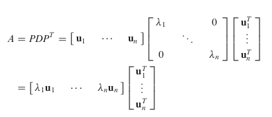
Using the column–row expansion of a product (Theorem 10 in Section 2.4), we can write

$$A = \lambda_1\textbf{u}_1\textbf{u}_1^T + \lambda_2\textbf{u}_2\textbf{u}_2^T + \cdots +\lambda_n\textbf{u}_n\textbf{u}_n^T \tag{2}$$

This representation of $A$ is called a spectral decomposition of A because it breaks up $A$ into pieces determined by the spectrum (eigenvalues) of $A$ .

• Each term in (2) is an $n \times n$ matrix of rank 1(번역본에서 계수 1).
  • For example, every column of $\lambda_1 \textbf{u}_1 \textbf{u}_1^T$ is a multiple of $\textbf{u}_1$.
• Furthermore, each matrix $\textbf{u}_j \textbf{u}_j^T$ is a projection matrix in the sense that for each $\textbf{x}$ in $\mathbb{R}^n$, the vector $(\textbf{u}_j \textbf{u}_j^T)\textbf{x}$ is the orthogonal projection(번역본에서 전사 이나 투영 이 개인적으로 나은듯) of $\textbf{x}$ onto the subspace spanned by $\textbf{u}_j$.

EXAMPLE 4

Construct a spectral decomposition of the matrix $A$ that has the orthogonal diagonalization

$$A=\begin{bmatrix}7&2\\2&4\end{bmatrix}=\begin{bmatrix}\frac{2}{\sqrt{5}}&\frac{-1}{\sqrt{5}}\\\frac{1}{\sqrt{5}}&\frac{2}{\sqrt{5}}\end{bmatrix}\begin{bmatrix}8&0\\0&3\end{bmatrix}\begin{bmatrix} \frac{2}{\sqrt{5}}&\frac{1}{\sqrt{5}}\\\frac{-1}{\sqrt{5}}&\frac{2}{\sqrt{5}}\end{bmatrix}$$

Solution

Denote the column of $P$ by $\textbf{u}_1$ and $\textbf{u}_2$. Then

$$A=8\textbf{u}_1\textbf{u}_1^T+3\textbf{u}_2\textbf{u}_2^T$$

To verify this decomposition of $A$, compute

$$\begin{aligned}\textbf{u}_1\textbf{u}_1^T &= \begin{bmatrix}\frac{2}{\sqrt{5}}\\\frac{1}{\sqrt{5}}\end{bmatrix} \begin{bmatrix}\frac{2}{\sqrt{5}}&\frac{1}{\sqrt{5}}\end{bmatrix}=\begin{bmatrix}\frac{4}{5}&\frac{2}{5}\\\frac{2}{5}&\frac{1}{5}\end{bmatrix}\\ \textbf{u}_2\textbf{u}_2^T &= \begin{bmatrix}\frac{-1}{\sqrt{5}}\\\frac{2}{\sqrt{5}}\end{bmatrix} \begin{bmatrix}\frac{-1}{\sqrt{5}}&\frac{2}{\sqrt{5}}\end{bmatrix}=\begin{bmatrix}\frac{1}{5}&\frac{-2}{5}\\\frac{-2}{5}&\frac{4}{5}\end{bmatrix} \end{aligned}$$

and

$$8 \textbf{u}_1\textbf{u}_1^T +3 \textbf{u}_2\textbf{u}_2^T = \begin{bmatrix}32/5 & 16/5 \\ 16/5 & 8/5 \end{bmatrix}+ \begin{bmatrix}3/5 & -6/5 \\ -6/5 & 12/5 \end{bmatrix}= \begin{bmatrix} 7 & 2 \\ 2 & 4 \end{bmatrix}=A \quad \blacksquare$$