ResNet: Deep Residual Learning for Image Recognition (2015)
ref.: original paper, Deep Residual Learning for Image Recognition
현재 많이 사용되는 구현 상 변화는 다음 논문을 참고하는게 더 나음:
- ref.: Bag of Tricks for Image Classification with Convolutional Neural Networks (He et al., CVPR 2019)
ILSVRC 2015 우승 모델이며, deep learning에서 “deep”의 의미를 크게 바꾼 모델임.
- Kaiming He, Xiangyu Zhang, Shaoqing Ren, Jian Sun이 제안함.
- ImageNet classification에서 top-5 error 3.57%를 기록함.
- 152 layers라는, 당시로서는 매우 놀라운 깊이의 deep model을 제안함.
ResNet은 skip connection 또는 shortcut connection을 도입한
Residual Block 을 사용하여
매우 깊은 모델의 학습 을 가능하게 함.
- ResNet은 identity mapping과 addition을 이용하는
shortcut connection을 통해residual learning을 수행 함. - 기존 plain network는 깊이가 증가하면 optimization이 어려워져 training error까지 증가하는 degradation problem이 나타날 수 있음.
- ResNet은 residual block 내부에 shortcut path를 추가 하여
깊은 network를 더 쉽게 optimize할 수 있도록 만듦. - 이후에는 addition 기반 residual connection뿐 아니라,
concatenation을 이용한 skip connection도 널리 사용(DenseNet)됨.
ResNet의
residual learning에서는 residual branch의 출력과 shortcut branch의 출력을 add 연산으로 결합함.
concatenation은 feature map을 channel 방향으로 이어 붙이는 방식임.
concatenation기반 연결은DenseNet (2017)을 통해 유용성을 보임.
concatenation 기반의 skip connection: DenseNet
concatenation을 사용한 DenseNet (2017)의 경우,
- low-level texture, edge, color pattern 같은 초기 feature가 뒤쪽 layer까지 직접 전달됨.
- concatenation 때문에 input width는 증가하지만, 각 layer가 새로 만들어내는 feature 수를 작게 유지하기 때문에 전체 parameter 수는 오히려 효율적으로 관리함.
- 병변의 미세한 색 변화, 경계, 표면 질감처럼 low-level feature가 중요한 의료 영상 데이터에서는 ResNet보다 높은 성능을 보일 수 있음.
- 추가적으로 DenseNet-121은 parameter efficiency 측면에서 소량 데이터에 유리할 수 있음.
- DenseNet-121은 대략 8M parameters 수준임.
- ResNet-50은 대략 25M parameters 수준임.
구조
각 종류별 구조는 다음과 같음:
- ResNet-18: [2, 2, 2, 2] Basic RU
- ResNet-34: [3, 4, 6, 3] Basic RU
- ResNet-50: [3, 4, 6, 3] Bottleneck RU
- ResNet-101: [3, 4, 23, 3] Bottleneck RU
- ResNet-152: [3, 8, 36, 3] Bottleneck RU
위 square bracket 에 있는 숫자는 각 stage별 Residual Unit 의 개수임.
18,34,50,101,152 라는 숫자는 ResNet 내의 conv와 FC layer들을 합친 trainable layer의 개수임.
이 전반적인 구조를 그림으로 나타내면 다음과 같음.
- Residual Unit (RU) 들이 반복되는 구조임.
위의 그림에선 입력을 처리하는 stem 이 위에 표시됨 (forward propagation: 위에서 아래)
Bullet list로 표현(아래에서 위로 표시)하면 다음과 같음:
StemResidual stagesRU (64ch, conv2_x): ResNet-18에선 2개의 convRU (128ch, conv3_x): ResNet-18에선 2개의 convRU (256ch, conv4_x): ResNet-18에선 2개의 convRU (512ch, conv5_x): ResNet-18에선 2개의 conv
Global Average PoolingFC classifier
ResNet의 입력 부분에는 본격적인 residual unit (RU)이 시작되기 전에 stem이 위치함.
stem은 입력 image를 초기 feature map으로 변환하는 부분임.- ImageNet용 ResNet에서는 일반적으로
7x7 convolution (64ch, stride=2)-BN-ReLU-3x3 max pooling (stride=2)로 구성됨. - 입력 image가 \(224 \times 224\)일 경우,
7x7 convolution을 지나면 spatial size가 \(112 \times 112\)가 됨. - 이후
3x3 max pooling을 지나면 spatial size가 \(56 \times 56\)가 됨. - 이 \(56 \times 56\), 64-channel feature map에서
RU (64ch)stage, 즉 논문 표기의conv2_x가 시작됨.
다음은 ResNet-34 와 VGG19를 비교한 그림임:
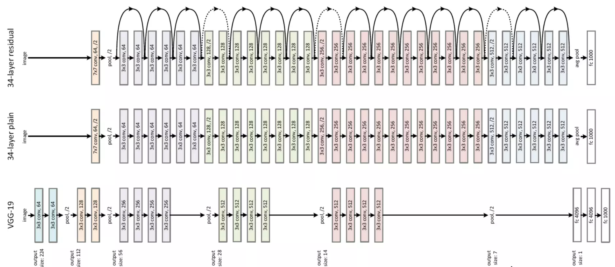
- stem과 residual stage, classifier 별로 다른 색을 사용함.
Residual stage는 많은 수의 convolutional layer가 residual unit (RU) 단위로 반복되어 구성됨.
- ResNet-18/34에서 사용하는
Basic RU는 보통 2개의 convolutional layers 로 구성됨.- 첫 번째 convolutional layer는 BN과 ReLU로 이어짐.
- 이후 두 번째 convolutional layer를 거치고, 그 결과는 BN을 통과함.
- 이 결과는 shortcut connection으로 전달된 input과 addition을 수행하고, 해당 결과는 다시 ReLU를 거침.
- ResNet-50/101/152에서 사용하는
Bottleneck RU는 3개의 convolutional layers 로 구성됨.1x1 convolution으로 channel 수를 줄임.3x3 convolution으로 spatial feature를 추출함.1x1 convolution으로 channel 수를 다시 확장함.
- 각
RU는 main path와 shortcut path를 함께 가지며,RU의 input과 output은 shortcut connection을 통해 연결됨.
ResNet의 기본 activation function은 ReLU이며, convolutional layer 뒤에서 BN (Batch Normalization)과 함께 사용됨.
파선(dotted shortcut)으로 그려진 skip connection 은 feature map의 spatial size나 channel 수가 바뀌어 \(\mathbf{x}\)와 \(\mathcal{h}(\mathbf{x})\)의 차원이 맞지 않는 경우를 의미함.
- 논문에서는 이를 zero-padding shortcut과 projection shortcut 의 두 가지 방식으로 구현하여 비교함.
- zero-padding shortcut 는 shortcut branch에서 identity mapping을 유지하되, channel 수가 늘어나는 부분을 0으로 padding함. 추가 parameter가 없음.
- projection shortcut 는 1x1 convolution을 사용하여 shortcut branch의 차원을 맞춤.
- projection shortcut이 대체로 더 우수한 결과를 보임.
- 현재
torchvision등에서 backbone으로 제공되는 대부분의 ResNet-18/34 basic block, ResNet-50/101/152 bottleneck block 구현은 차원이 바뀌는 지점에서 projection shortcut을 사용 함.
stage가 바뀌는 경우에는 pooling 대신 convolution에서 stride=2를 사용하여 spatial size를 줄이는 것이 일반적임.
- 예를 들어
RU (64ch)stage, 즉 논문 표기의conv2_x에서RU (128ch)stage, 즉conv3_x로 넘어갈 때, - spatial size는 \(56 \times 56\)에서 \(28 \times 28\)로 줄어듦.
- channel 수는 \(64\)에서 \(128\)로 늘어남.
- 이때 width와 height가 각각 ½로 줄어들기 때문에 spatial area는 ¼이 됨.
ResNet은 주로 convolutional layer와 fully-connected layer만 layer 수로 count함.
즉, BN, ReLU, pooling layer 등은 layer 수에 포함하지 않음.
ResNet-34:
Conv (64ch)-RU (64ch, conv2_x)\(\times 3\) -RU (128ch, conv3_x)\(\times 4\) -RU (256ch, conv4_x)\(\times 6\) -RU (512ch, conv5_x)\(\times 3\) -FC (1000ch)
ResNet-152:
Conv (64ch)-Bottleneck RU (256ch, conv2_x)\(\times 3\) -Bottleneck RU (512ch, conv3_x)\(\times 8\) -Bottleneck RU (1024ch, conv4_x)\(\times 36\) -Bottleneck RU (2048ch, conv5_x)\(\times 3\) -FC (1000ch)
Residual Block
- 다음은 ResNet-18/34에서 사용된
Basic RU (RU = Residual Unit)와, - 그보다 더 깊은 ResNet에서 사용된
Bottleneck RU의 구성임.
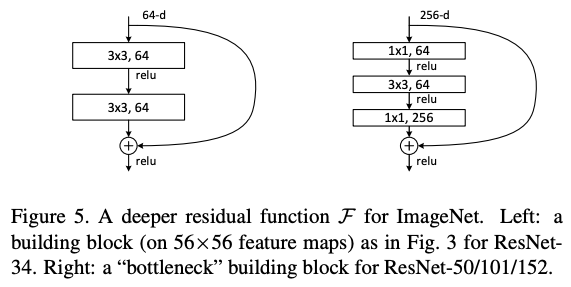
- 왼쪽의
Basic RU는 ResNet-18/34에서 사용됨. - 오른쪽의
Bottleneck RU는 ResNet-50/101/152에서 사용됨. - 기본
RU는 2개의 3x3 convolution으로 구성됨. Bottleneck RU는 1x1, 3x3, 1x1 convolution으로 구성됨.- 첫 번째 1x1 convolution은 channel 수를 줄이는 역할을 함.
- 3x3 convolution은 줄어든 channel 수에서 spatial feature를 추출함.
- 마지막 1x1 convolution은 channel 수를 다시 확장함.
Connection
다음은 Basic RU에서 identity shortcut과 projection shortcut을 보여줌.
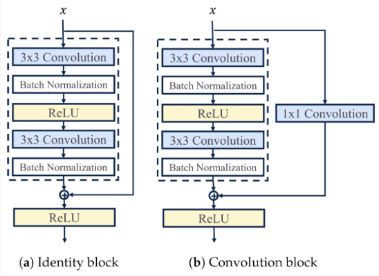
- 2개의 conv 를 사용하는
Basic RU임. - main branch의 구성이
Bottleneck RU에선 앞서 보인 3개의 conv 를 사용. - 오른쪽의 projection connection은 downsampling용으로 앞서 3x3 conv에서 stride=2를 사용함.
identity shortcut
input과 main branch output의 shape이 동일한 RU에서 사용함.
- stride=1로 spatial resolution의 변화가 없고
- channel 수도 동일한 경우
- 별도의 convolution 없이 input을 그대로 더함.
projection shortcut
input과 main branch output의 shape이 다른 경우 사용함.
- stage 전환에서 stride=2로 downsampling하는 경우
- 또는 Bottleneck RU처럼 channel 수가 변경되는 경우
1x1 convolution을 사용하여 shortcut의 shape을 main branch output에 맞춤.
다음의 오른쪽이 ResNet-18의 downsampling RU의 구조임:
Variations of RU
ResNet에는 여러 variation 들이 있음:
- ResNet-B 는 torchvision 의 resnet 구현물에 도입됨 (
timm의 구현물도 마찬가지)- Path A의 1x1 conv w/ stride=2가 input feature map의 ¾를 무시하게 되기 때문에,
- 이를 방지하기 위해 downsampling block에서 path A의 첫 두 conv block의 구조를 변경
- ResNet-C는 ResNet-B의 downsampling block 구조를 포함.
- 그리고 input stem의 7x7 conv를 3x3 conv 3개로 변경
- 이를 deep stem 이라고도 함.
- inception-v2 에서 제안됨.
- ResNet-D는 ResNet-B의 downsampling block에서 사용한 path A 구조와 ResNet-C의 input stem 구조를 포함.
- Path B의 1x1 conv를 avgpool + 1x1 conv 구조로 변경
- 이유는 1x1 conv w/ stride 2 의 information loss 때문임
- ResNet-D 의 경우
timm.resnet50d와 같이d가 뒤에 붙는 이름을 가짐.
Residual Learning
기존 모델이 hypothesis \(\mathcal{H}(\mathbf{x})\)를 직접 학습하는 것과 달리, ResNet은 hypothesis와 input \(\mathbf{x}\)의 차이인 residual function을 학습함.
- 기존 plain network의 어떤 block이 입력 \(\mathbf{x}\)를 받아 원하는 mapping \(\mathcal{H}(\mathbf{x})\)를 직접 학습한다고 생각할 수 있음.
- ResNet은 이 mapping을 직접 학습하는 대신, residual function \(\mathcal{F}(\mathbf{x})\) 을 학습하도록 문제를 바꿈.
따라서 원하는 mapping은 다음과 같이 다시 표현할 수 있음.
여기서 중요한 점은 ResNet이 \(\mathcal{H}(\mathbf{x})\)를 먼저 구한 뒤 \(\mathbf{x}\)를 빼는 방식으로 동작하는 것이 아니라는 점임.
- main path의 convolutional layers가 직접 \(\mathcal{F}(\mathbf{x})\)를 학습함.
- shortcut path는 \(\mathbf{x}\)를 그대로 전달함.
- 두 path의 결과를 addition하여 block의 출력을 만듦.
차원이 같은 경우 residual block의 출력은 다음과 같이 표현됨.
차원이 다른 경우에는 shortcut branch에도 projection을 적용할 수 있음.
- \(\{W_i\}\)는 residual branch의 convolutional weights
- \(W_s\)는 shortcut branch의 projection weight임.
Residual learning의 핵심 직관은 다음과 같음.
- 어떤 block에서 이상적인 mapping이 identity mapping에 가깝다면, plain network는 \(\mathcal{H}(\mathbf{x}) \approx \mathbf{x}\)를 직접 학습해야 함.
- ResNet에서는 residual branch가 \(\mathcal{F}(\mathbf{x}) \approx 0\)에 가까운 값을 학습하면 됨.
- 즉, identity mapping이 필요한 경우에는 residual branch가 거의 아무 변화도 주지 않도록 학습하면 되므로 optimization이 쉬워질 수 있음.
- 이 때문에 ResNet은 깊이가 크게 증가해도 plain network보다 학습이 안정적으로 이루어질 수 있음.
torchvision
최근 torchvision에서는 pretrained=True 대신 weights argument 사용이 권장됨.
from torchvision.models import resnet50, ResNet50_Weights

model = resnet50(weights=ResNet50_Weights.DEFAULT)
````

다른 ResNet 계열 모델도 같은 방식으로 사용할 수 있음.

```python
from torchvision.models import resnet18, ResNet18_Weights
from torchvision.models import resnet34, ResNet34_Weights
from torchvision.models import resnet101, ResNet101_Weights
from torchvision.models import resnet152, ResNet152_Weights
from torchvision.models import wide_resnet50_2, Wide_ResNet50_2_Weights
from torchvision.models import wide_resnet101_2, Wide_ResNet101_2_Weights

model = resnet18(weights=ResNet18_Weights.DEFAULT)
model = resnet34(weights=ResNet34_Weights.DEFAULT)
model = resnet101(weights=ResNet101_Weights.DEFAULT)
model = resnet152(weights=ResNet152_Weights.DEFAULT)
model = wide_resnet50_2(weights=Wide_ResNet50_2_Weights.DEFAULT)
model = wide_resnet101_2(weights=Wide_ResNet101_2_Weights.DEFAULT)