Convolution
이 문서에서의 convolution은 digital image processing등에서의 convolution을 다루고 있음.
signal processing의 discrete convolution에 대한 건 다음 문서를 참고할 것:
Discrete Convolution,
Circular ConvolutionDeep Learning의 Convolution Layer에 대한 보다 자세한 건 다음 문서를 참고할 것:
Convolution Layer
image filtering에서 spatial domain filtering은 주로
- filter 또는
- kernel 또는
- window 라고
불리는 행렬(=impulse response)과 입력 영상의 Convolution 으로 이루어짐.
Convolution (합성곱)은 기호 ⊗ or ∗ 등으로 표기되지만 통일된 기호는 없음.
- 어찌보면, spatial operation의 끝판왕이라고 봐도 됨.
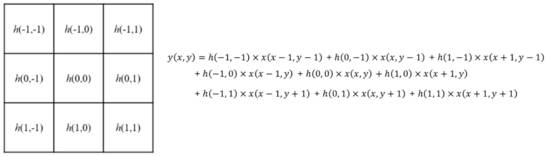
convolution의 수식은 다음과 같음.
where
- \(h(x,y)\) : filter or kernel
- \(f(x,y)\) : original image
- \(g(x,y)\) : output image
convolution은
- cross-correlation과 달리 교환법칙이 성립 하며,
- impulse response(영상에선 point spread function)와 입력 신호를 이용하여 시스템의 response를 구하는 연산 임.
Cross correlation은 매우 유사하지만, 두 신호의 유사도를 얻기 위해 사용됨.
- cross-correlation과 달리 입력 함수 중 하나가 reflection이 이루어진다는 차이가 있음.
- cross-correlation에 대한 보다 자세한 내용은 다음 url을 참고 : Cross correlation
하지만, 이미지 처리에서는 대부분 kernel을 대칭적인 것을 사용하다 보니 cross-correlation과 차이가 없는 경우가 많고, 특히 ML(기계학습)이나 DL(딥러닝)에서 kernel이 이미 상하좌우로 flip하여 입력하면 된다는 가정 하에 convolution의 구현이 실제로는 cross-correlation인 경우가 대다수임.
Kernel (or Filter, Mask, Window)
- 유한한 크기의
impulse response(or point spread function)의 특성 계수 - 시스템 응답 특성 계수를 가지고 있는 matrix 혹은 tensor임.
DL등에서 convolution layer은 위의 2D kernel이 아닌 3D kernel로 구성되는 게 일반적임. (channel이 보통 3이므로 raw image를 입력으로 삼는 경우 kernel size의 3개의 matrix를 가지고 있다고 생각하면 됨.)
- kernel의 width와 height를 통해 local receptive field의 크기가 결정됨.
- receptive field란 convolution의 결과로 나오는 feature map의 한 pixel(or voxel)의 값을 만드는데 관여한 input map(or image)의 영역을 의미함.
Convolution 수행 방식
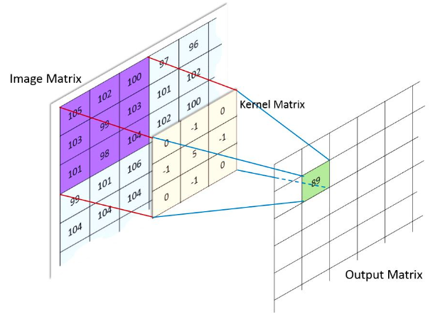
위의 그림에서 Kernel matrix는 상하좌우로 뒤집힌(reflection) 상태임. (Cross correlation과 차이)
- 다시 강조하지만, DIP나 ML, DL에서는 cross-correlation과 거의 구분하지 않음.
아래 그림은 다채널의 입력에 대해, 2개의 filter (or kernel)이 주어져서 convolution이 이루어지는 과정을 보여주고 있음.
- \(5 \times 5 \times 3\) image를 상하좌우로 1씩 padding을 수행하고,
- \(3 \times 3\) kernel을(엄밀하게는 \(3\times 3\times 3\)) 통해 convolution을 수행하여 \(3 \times 3 \times 2\) image를 얻어냄.
- Kernel은 2 pixels의
stride를 사용하여 이동함. - 결과 영상의 depth \(2\)는 kernel (or filter)이 2개 (
W0,W1) 사용됨을 의미함.
Stride
Convolution을 수행할 때, stride는 일종의 sub-sampling factor로 동작함.
이는 stride가 클수록 결과 feature map의 사이즈가 줄어들게 되며, DL에서 convolution layer의 computational complex를 효과적으로 낮출 수 있도록 해준다. Kernel이 sliding을 통해 적용되어나가는데, stride는 어느 간격으로 Kernel이 sliding될지를 나타낸다. (stride가 클수록 듬성듬성 처리된다고 생각할 수 있음.)
다음은 stride가 \(2 \times 2\)인 경우(오른쪽으로 sliding할 때 2pixels, 아래로 sliding 할 때도 2pixels)임. (stride가 1인 경우 \(3\times 3\) feature map이 나오는 것과 달리 이 경우 \(2 \times 2\) feature map이 결과임)
- \(5 \times 5\) 입력에 \(2\times 2\) stride로 \(3\times 3\) kernel로 Convolution.
- 상단의 녹색 matrix가 출력임.
Padding
convolution의 경우, padding하지 않는다면 출력이 입력보다 작은 크기(폭과 높이)가 되게 된다.
- Convolution을 수행할 때, Padding이 없을 경우 주변부는 결과에 영향력이 줄어들게 된다.
- Kernel이 제대로 놓여지기 어려운 위치가 주변부이기 때문임.
- 때문에 Convolution을 하기 전에 영상에 Padding을 수행하는게 일반적임.
결과 영상 크기
Padding과 Stride, Kernel의 크기에 따른 출력의 크기는 다음과 같음:
Pillow 에서 convolution 활용
PyTorch 의 nn.Conv2D를 이용한 convolution 활용
OpenCV를 통한 convolution
OpenCV 는 filter2D를 통해 convolution을 제공.
src: input imageddepth: output image dtype :-1인 경우 input image와 동일한dtype를 가짐. /CV_8U,CV_16U,CV16S,CV_32F,CV_64Fkernel: kernel or window or mask or filter matrixdst: output imageanchor: kernel의 기준점. 결과값이 치환될 위치. default (-1,-1) 로 kernel의 중앙을 의미delta: 결과값에 추가할 값.borderType: padding 형태 (기본으로BORDER_REFLECT_101임).
간단한 예제 코드는 다음과 같음.
#img = cv2.imread('./data/lena.jpg')
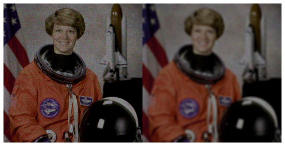
img = astro_noise.copy() # 아래 예는 poisson noise를 가함.
print(img.dtype, img.shape)
k_size = 10
kernel = np.full((k_size,k_size),1./(k_size**2))
blurred = cv2.filter2D(img, -1, kernel)
print(f'from {img.shape} to {blurred.shape}')
plt.figure(figsize=(10,20))
plt.imshow(np.concatenate((img,blurred),axis=1))
plt.axis('off')
plt.show()
결과는 다음과 같음.