Morphological Operations¶

Introduction¶

Morphology 는 형태학 을 의미.

Morphology means the study of the shape and structure of living things from a biological perspective.
Morphology is a discipline of biology related to the study of the shape and structure of the organism and its unique structural characteristics.

생물학자들이 동식물이 보여주는 모양 및 구조을 지칭하고 분류하는 것에서 유래.

DIP에서는

noise(작은 크기의) 제거,
구멍 메우기,
연결이 끊어진 선(line)을 이어주기,
boundary 추출 등에서 이용되는 shape(형태)에 기반한 연산 을 가르킴.

간략히 정리하면 영상처리(or Computer vision)에서 다음의 연산들을 가르킴.

Object의 모양(Structure, shape)을 분석 하는데 사용되는 연산.
Object의 모양을 원하는 형태로 변경 하는데 사용되는 연산.

대상에 따라,

binary morphology(w/ binary image)와

contrast morphology(w/ grayscale image) 로 나뉨.

영상처리에서 Morphology¶

“Binary image와 gray scale image의 기하학적 구조 를 분석 처리하는 기법” 을 가르킴.

Binary image : 기하학적 구조가 바뀜.
Gray scale image : 직접적으로는 pixel의 값이 변경되면서 전체 영상내 object의 모양 및 구조 가 변경됨.

OpenCV Tutorial에서 설명하고 있는 Morphology Operation은 다음과 같음

Morphological transformations are some simple operations based on the image shape.

It is normally performed on binary images .

It needs two inputs,

one is our original image,

second one is called structuring element or kernel which decides the nature of operation.

Two basic morphological operators are Erosion and Dilation.

Then its variant forms like Opening, Closing, Gradient etc also comes into play.

주로 Image 내의 object들의 구조 및 모양 에 기반한 처리임.

경계, 골격구조, convex-hull (주어진 점들을 모두 포함하는 최소 크기의 다각형) 등의 object의 기하학적 구조 관련 feature를 처리 하는데 사용됨.
Object의 기하학적 구조에 대한 description을 생성 하는데 사용됨.

대표적인 연산으로는 다음 2가지 있음.

Erosion (침식)
Dilation (팽창)

응용분야로는

Morphology filtering
Thinning (~세선화)
Pruning 등등

Basic Operations¶

Morphological Operations는 주로 화소집합 을 다루며, 때문에 set(집합)에서의 연산들을 기본 연산으로 사용한다.

Basic Operations (on a binary image) for Morphological Operation

Structuring Element (SE, 구조요소, 구조화요소)¶

Morphological operation의 동작특성을 결정짓는 입력으로, spatial filtering의 kernel과 유사함.

일종의 0과 1로 이루어진 kernel로 볼 수 있음.
SE에서 1인 영역에 대응되는 target image(대상영상)의 pixel의 값(Binary image의 경우 1 or 0)에 따라, Structuring Element의 anchor 위치(주로 중앙, origin이 anchor에 해당)에 해당하는 pixel(일반적으로 SE의 중심에 해당하는 pixel)의 값이 결정됨.
종류
- cv2.MORPH_RECT
- cv2.MORPH_ELLIPSE
- cv2.MORPH_CROSS

cv2.MORPH_RECT 는 네모(Rectangle) 모양의 kernel임.
다음 코드는 해당 kernel을 \(5\times5\) 로 생성.

# Rectangular Kernel
kernel = cv2.getStructuringElement(cv2.MORPH_RECT,(5,5))
print(kernel)

결과는 다음과 같음.

[[1 1 1 1 1]
 [1 1 1 1 1]
 [1 1 1 1 1]
 [1 1 1 1 1]
 [1 1 1 1 1]]

cv2.MORPH_ELLIPSE 는 타원(circle도 포함) 모양의 kernel임.
다음 코드는 해당 kernel을 \(10\times 15\) 로 생성.

# Elliptical Kernel
kernel = cv2.getStructuringElement(cv2.MORPH_ELLIPSE,(15,10))
print(kernel)
plt.imshow(kernel, cmap='gray')

결과는 다음과 같음.

[[0 0 0 0 0 0 0 1 0 0 0 0 0 0 0]
 [0 0 0 1 1 1 1 1 1 1 1 1 0 0 0]
 [0 1 1 1 1 1 1 1 1 1 1 1 1 1 0]
 [0 1 1 1 1 1 1 1 1 1 1 1 1 1 0]
 [1 1 1 1 1 1 1 1 1 1 1 1 1 1 1]
 [1 1 1 1 1 1 1 1 1 1 1 1 1 1 1]
 [1 1 1 1 1 1 1 1 1 1 1 1 1 1 1]
 [0 1 1 1 1 1 1 1 1 1 1 1 1 1 0]
 [0 1 1 1 1 1 1 1 1 1 1 1 1 1 0]
 [0 0 0 1 1 1 1 1 1 1 1 1 0 0 0]]

cv2.MORPH_CROSS 는 십자 모양의 kernel임.
다음 코드는 해당 kernel을 \(5\times 5\) 로 생성.

# Cross-shaped Kernel
kernel = cv2.getStructuringElement(cv2.MORPH_CROSS,(5,5))
print(kernel)
plt.imshow(kernel)

결과는 다음과 같음.

[[0 0 1 0 0]
 [0 0 1 0 0]
 [1 1 1 1 1]
 [0 0 1 0 0]
 [0 0 1 0 0]]

OpenCV에서 기본으로 제공하는 위의 kernels 외에도
Numpy를 이용하여 고유한 kernel을 만들어 사용하는 것도 가능함.

Erosion (침식)¶

Erosion의 경우,

Structuring Element가 convolution의 kernel처럼
입력영상의 전영역에 걸쳐 sliding되면서 결과 영상이 나옴.

Erosion의 수식은 다음과 같음.

\[ f\ominus \text{s}= \{o(\textbf{z})|(\textbf{s})_\textbf{z} \subseteq f\} \]

where

\(f\) : input image
\(\text{s}\) : Structuring Element
\(\textbf{z}\) : SE를 \(\textbf{z}\)만큼 translation. SE가 이동된 위치를 나타내는 vector.
\(o(\textbf{z})\) : 결과 영상에서 \(\textbf{z}\) 위치의 pixel intensity. SE가 입력영상의 subset이거나 같으면 1이고, 아니면 0.

SE가 input image의 subset인 경우에 anchor pixel은 1!

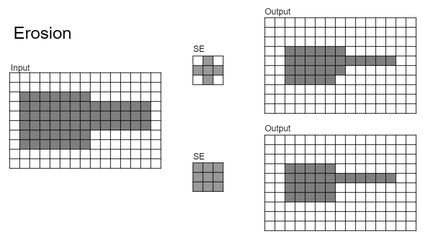
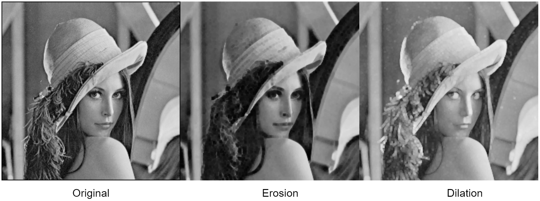
Erosion의 효과는 다음과 같음.

Object의 크기는 축소 됨(binary image) → Background(배경)은 확장됨.
작은 돌출부 제거 및 크기가 작은 noise 제거
- 단점으로는 작은 크기의 object도 제거됨 .
- noise 수준의 작은 크기인 object도 제거되는 단점 존재.
연결성 약화 (별개의 객체인데 맞닿아 있는 경우 떨어지게 됨)
주변에 비해 높은 값을 가지는 noise 제거(gray-scale image)

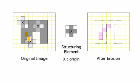
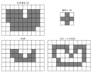
Erosion : ref. KOCW

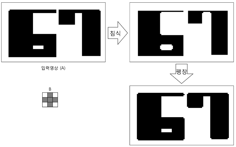
Example 1
- 이 예제에서는 어두운 부분이 255(or 1)에 해당하고, 흰색이 0에 해당함.
- Object (pixel의 값이 1)의 크기가 줄어드는 것을 확인할 수 있음.
- 보다 큰 크기의 SE를 사용할수록 Erosion의 효과가 커짐.
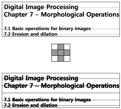
Example 2
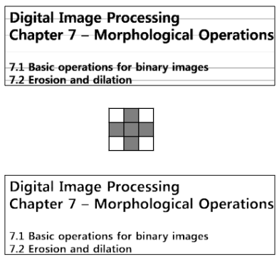
- 이 예제에서는 어두운 부분이 255(or 1)에 해당하고, 흰색이 0에 해당함.
- Object(글자)들의 경계가 침식되어 세선화(thinning) (object의 크기가 줄었다고 볼 수 있음) 됨.
- 가로 방향의 가는 선분들 제거
- 글자에 속하는 pixel들의 경우, SE(구조요소)에 따른 erosion(침식)의 강도가 다소 낮기 때문에, 전체적인 object의 구조가 상대적으로 잘 보존됨.
- SE(구조요소) 보다 더 작은 부분을 잡음으로 처리 하여 제거하고, 그렇지 않은 부분은 형태의 주요 요소로 보고 가급적 그 형태를 유지(boundary의 부분은 제거되어 object의 크기가 줄어들게된다).

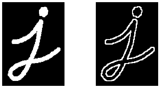
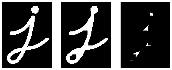
다음 코드는 OpenCV Tutorial에서 제공한 예로, Numpy의 ndarray로 만든 rect kernel로 erosion 을 수행한 결과임.

import cv2
import numpy as np
import matplotlib.pyplot as plt

img = cv2.imread('./images/j.png',0)

kernel = np.ones((5,5),np.uint8)
print(kernel)

erosion = cv2.erode(img,kernel,iterations = 1)
plt.figure(figsize=(10,5))
plt.subplot('121')
plt.imshow(img,cmap='gray'), plt.axis('off')
plt.subplot('122')
plt.imshow(erosion,cmap='gray'), plt.axis('off')

사용한 j.png는 다음 url에서 다운로드 가능 : j.png

결과 이미지는 다음과 같음.

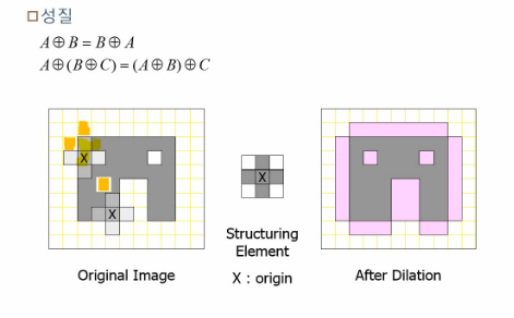
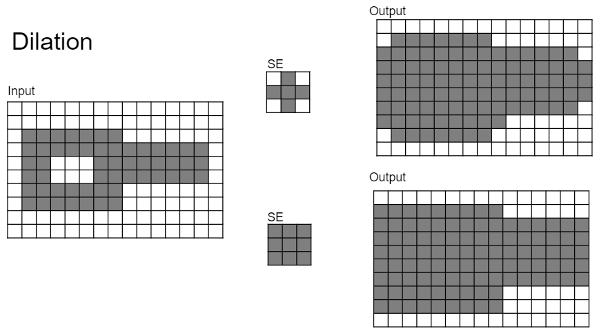
Dilation (팽창)¶

Erosion의 경우처럼, Structuring Element가 convolution의 kernel처럼 입력영상의 전영역에 걸쳐 sliding되면서 결과 영상이 나옴.

Dilation의 수식은 다음과 같음.

\[ f\oplus \text{s}= \{o(\textbf{z})|(\textbf{s})_\textbf{z} \cap f \ne \emptyset \} \]

where

\(f\) : input image
\(\text{s}\) : Structuring Element
\(\textbf{z}\) : SE를 \(\textbf{z}\)만큼 translation. SE가 이동된 위치를 나타내는 vector.
\(o(\textbf{z})\) : 결과 영상에서 \(\textbf{z}\) 위치의 pixel intensity. SE와 입력영상의 interception이 empty set이면 0, 아니면 1

SE와 intersection이 null이 아니면, anchor pixel은 1이 된다.

Dilation의 효과는 다음과 같음.

Object 의 크기가 증가 함(binary image) → 배경은 축소
작은 구멍들을 메꿈.
연결성 강화 (연결된 선이 끊어져보일때 연결해줌)
- 근접한 object들이 연결되게 됨.
주변에 비해 낮은 값을 가지는 noise 제거(gray-scale image의 경우)

Example 1
- 이 예제에서는 어두운 부분이 255(or 1)에 해당하고, 흰색이 0에 해당함.
Example 2
- 이 예제에서는 어두운 부분이 255(or 1)에 해당하고, 흰색이 0에 해당함.
- Object 영역의 확장
- 가로 방향으로의 가는 선분들이 두꺼워짐 ← 연결성 강화.

OpenCV에서 dilation은 cv2.dilate 함수로 제공된다. 다음 코드는 이를 간단히 사용한 예를 보여준다.

dilation = cv2.dilate(img,kernel,iterations = 1)
plt.figure(figsize=(10,5))
plt.subplot('121')
plt.imshow(img,cmap='gray'), plt.axis('off')
plt.subplot('122')
plt.imshow(dilation,cmap='gray'), plt.axis('off')

erosion에서 사용한 SE kernel를 다시 사용함.

결과는 다음과 같음.

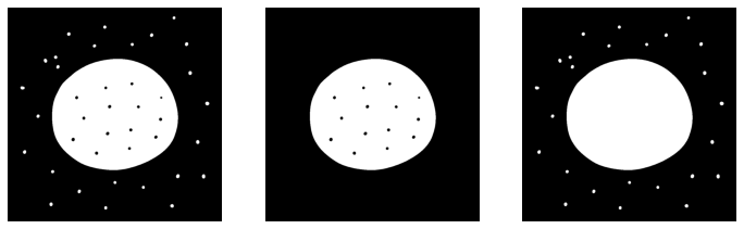
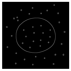
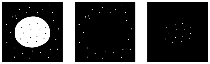
Erosion vs. Dilation on the Binary Image¶

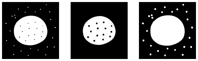
Left: original, Center: erosion, Right: dilation

가운데의 erosion의 결과는 내부의 hole이 커지는 대신, 외부의 작은 점들은 사라짐.
오른쪽의 dilation의 결과는 내부의 hole이 메꾸어진 대신, 외부이 작은 점들의 크기가 커짐.

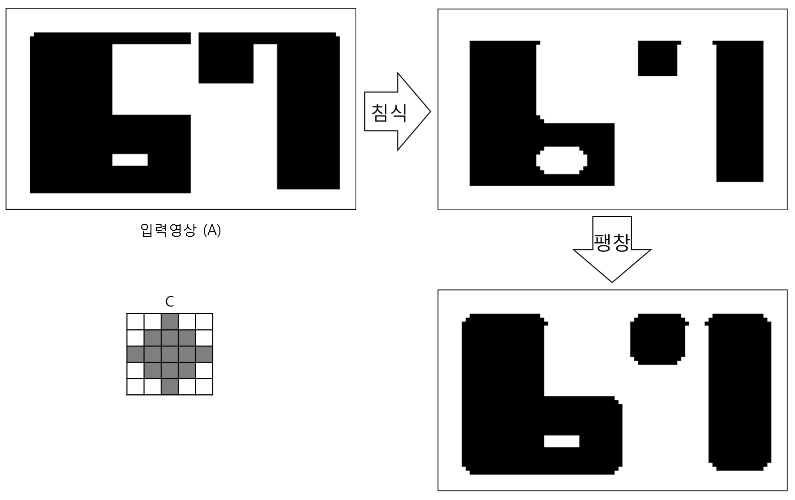
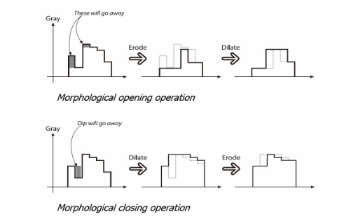
Opening¶

💡 Erosion 수행 후 Dilation

\[ f\circ \text{s} =(f \ominus \text{s})\oplus \text{s} \]

연산 부호의 원이 비어있음 (open)

Erosion 의 단점인 object 크기가 줄어드는 문제를 해결 .

주변보다 밝은 noise 제거 및 맞닿아있는 객체 분리, 돌출된 작은 영역 제거에 사용됨.
주된 효과는 Erosion 이며, object가 작아지는 문제를 개선! (개선된 erosion)
Example 1
- 이 예제에서는 어두운 부분이 255(or 1)에 해당하고, 흰색이 0에 해당함.
- 모서리들이 부드러워졌으나, 원래 영상의 모양에서 큰 변화가 없음. 주의할 건 SE의 크기가 지나치게 커지면 상대적으로 작은 크기의 구조가 제거됨.(아래의 example2참고)
Example 2
- 이 예제에서는 어두운 부분이 255(or 1)에 해당하고, 흰색이 0에 해당함.
- Morphological Operation에서 적절한 SE (크기나 모양)가 아닌 경우, 원하는 처리가 이루어지지 않음.

opening은 기본연산인 erosion과 dilation의 조합에 의한 일종의 extended operation으로 OpenCV에서는 cv2.morphologyEx함수를 통해 제공됨.

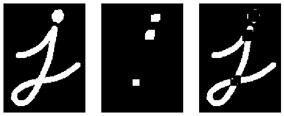
아래의 예제는 OpenCV Tutorial에서 제공된 예제코드로
salt and pepper noise에서 salt 만을 가한 image (또는 impulse noise라고 볼 수 있음)에 대해
opening을 통해 해당 impulse noise(or salt noise)를 제거하는 예제임.

row,col = img.shape
s_vs_p = 1 #0.5
amount = 0.01
out = np.copy(img)

# Salt mode
num_salt = np.ceil(amount * img.size * s_vs_p)
coords = [np.random.randint(0, i, int(num_salt))
          for i in img.shape]
out[tuple(coords)] = np.max(img)

# Pepper mode
num_pepper = np.ceil(amount* img.size * (1. - s_vs_p))
coords = [np.random.randint(0, i, int(num_pepper))
          for i in img.shape]
out[tuple(coords)] = np.min(img)

print(img.dtype)
# kernel = np.ones((3,3),np.uint8)        
opening = cv2.morphologyEx(out, cv2.MORPH_OPEN, kernel)

plt.figure(figsize=(10,5))
plt.subplot('121')
plt.imshow(out,cmap='gray'), plt.axis('off')
plt.subplot('122')
plt.imshow(opening,cmap='gray'), plt.axis('off')

앞서 사용한 SE kernel을 재사용한 경우와 \(3\times 3\) shape의 kernel로 변경해서 동작시켜 볼 것.

결과는 다음과 같음.

Closing¶

💡 Dilation 수행 후 Erosion

\[ f\bullet\text{s}=(f\oplus \text{s})\ominus \text{s} \]

연산부호의 원이 꽉 차 있음(close)

Dilation 의 단점인 object의 크기가 커지는 문제를 해결.

주변보다 어두운 noise 제거(hole을 채움) 및 끊어진 부분 연결에 사용됨.
전체적인 윤곽 파악 에 이용됨.
- 조명 등으로 인한 조도차로 object의 구멍이 난 것처럼 보이는 문제점을 해결
주된 효과는 Dilation이며, dialation의 부작용인 object가 커지는 문제를 해결.
Example 1
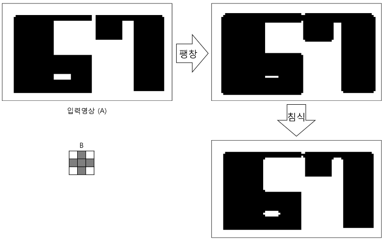
- 이 예제에서는 어두운 부분이 255(or 1)에 해당하고, 흰색이 0에 해당함.
Example 2
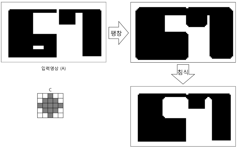
- 이 예제에서는 어두운 부분이 255(or 1)에 해당하고, 흰색이 0에 해당함.

closing도 기본연산인 erosion과 dilation의 조합에 의한 확장 연산으로
OpenCV에서는 cv2.morphologyEx함수를 통해 제공됨.

아래의 예제는 OpenCV Tutorial에서 제공된 예제코드로 salt and pepper noise에서 pepper noise만을 가하고 이를 closing을 통해 제거하는 예제임.

image에 구멍이 난 것처럼 보임 (주변보다 낮은 값을 가지는 noise)

row,col = img.shape
s_vs_p = 0.0 #1.0
amount = 0.01
out = np.copy(img)
# Salt mode
num_salt = np.ceil(amount * img.size * s_vs_p)
coords = [np.random.randint(0, i, int(num_salt))
          for i in img.shape]
out[tuple(coords)] = np.max(img)

# Pepper mode
num_pepper = np.ceil(amount* img.size * (1. - s_vs_p))
coords = [np.random.randint(0, i, int(num_pepper))
          for i in img.shape]
out[tuple(coords)] = np.min(img)

print(img.dtype)
#kernel = np.ones((3,3),np.uint8)        
closing = cv2.morphologyEx(img, cv2.MORPH_CLOSE, kernel)

plt.figure(figsize=(10,5))
plt.subplot('121')
plt.imshow(out,cmap='gray'), plt.axis('off')
plt.subplot('122')
plt.imshow(closing,cmap='gray'), plt.axis('off')

결과는 다음과 같음.

Opening vs. Closing on the Binary Image¶

Left: original, Center: Opening, Right: Closing

앞서 erosion과 dilation만을 가한 경우에 비해, image가 축소 또는 확대되지 않는 것을 확인 가능함.
opening에서는 주변보다 큰 값을 가지는 작은 크기의 noise를 제거.
closing에서는 주변보다 작은 값을 가지는 작은 크기의 noise를 제거.

Opening vs. Closing on the Gray-scale Image¶

Morphological Operations가 주로 binary image에서 사용되나 gray-scale image에서도 사용 가능하다.

Erosion on the gray-scale image¶

Gray-scale image에서의 erosion은 다음과 같음.

임의의 위치의 pixel value를 기준으로
Structure element와 겹쳐지는 영역 내 pixel에 대해
“pixel의 각 값”과 대응하는 “SE의 값”을 빼고,
그 결과 중 가장 작은 것 을 선택함.

수식은 다음과 같음.

\[ f\ominus\text{s}=\text{min}\{f(x+m,y+n)-\text{s}(m,n)|(x+m),(y+n)\in D_f \text{ and }m,n\in D_\text{s}\} \]

where

\(D_f\): 입력영상 \(f\)의 pixel 좌표 들의 집합.
\(D_\text{s}\) : SE \(\text{s}\)의 pixel 좌표 들의 집합.

Dilation on the gray-scale image¶

Gray-scale image에서의 dilation은 다음과 같음.

임의의 위치의 pixel value를 기준으로
SE와 겹쳐지는 영역 내 pixel에 대해
“pixel의 각 값”과 대응하는 “SE의 값”을 더하고,
그 결과 중 가장 큰 것 을 선택함.

수식은 다음과 같음.

\[ f\oplus \text{s}=\text{max}\{f(x+m,y+n)+\text{s}(m,n)|(x+m),(y+n)\in D_f \text{ and }m,n\in D_\text{s}\} \]

where

\(D_f\): 입력영상 \(f\)의 pixel 좌표 들의 집합.
\(D_\text{s}\) : SE \(\text{s}\)의 pixel 좌표 들의 집합.

Examples of gray-scale image¶

Gray-scale image에서
Erosion은 주변보다 높은 값들을 낮게 만들고 (=깍아냄)
Dilation은 주변보다 낮은 값들을 높게 만들어냄 (=부풀림)

Untitled

Erosion : 상대적으로 크기가 작은 밝은 영역이 제거(어두워짐)되고 전체적으로 어두워짐 (min).
Dilation : 상대적으로 크기가 작은 어두운 영역이 제거(밝아짐)되고 전체적으로 밝아짐 (max).
위에서 사용된 SE는 3x3의 박스 (1로 채워진)임.

Opening and Closing¶

Gray-scale에서의 opening과 closing은
binary image에서와 같이,
각각 erosion과 dilation을 개선한 연산임.

Opening

상대적으로 크기가 작은 밝은 상세 부분은 제거됨.
상대적으로 크기가 큰 밝은 부분은 pixel value가 유사하게 유지됨.

Closing

상대적으로 크기가 작은 어두운 상세 부분이 제거됨.
상대적으로 크기가 큰 어두운 부분은 pixel value가 유사하게 유지됨.

다음 그림은 opening과 closing의 횩과를 보여준다.

Untitled

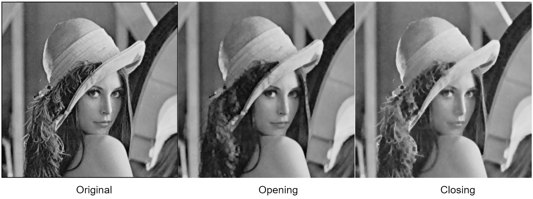
전체적으로 영상의 intensity가 다르게 되는 문제점을 opening과 closing은 개선하고 있음.
erosion과 dilation 만을 가해준 경우에 비해, 원본의 주요 정보를 잘 유지해준다.

Gradient¶

Dilation과 Erosion을 이용한 확장 연산 중 하나임.
(spatila filtering의 gradient와 구분할 것. 단, 효과는 유사!)

💡 Dilation - Erosion

Boundary Detection 이 가능함.

gradient도 확장 morphological operation이며 사용법은 opening과 closing과 유사함.

gradient = cv2.morphologyEx(img, cv2.MORPH_GRADIENT, kernel)

plt.figure(figsize=(10,5))
plt.subplot('121')
plt.imshow(img,cmap='gray'), plt.axis('off')
plt.subplot('122')
plt.imshow(gradient,cmap='gray'), plt.axis('off')

위 코드의 결과는 다음과 같음.

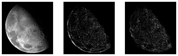
Erosion 기반의 Boundary Detection¶

사실 dilation에서 erosino을 빼는 gradient 외에도 Boundary Detection은 가능함.

Object 영상 과 그 Object 영상의 Erosion(침식) 영상 간의 Difference 연산 으로도 boundary를 구할 수 있음.

Erosion(침식)의 결과는 객체의 경계선이 깎인 형태
입력 객체와 Erosion의 결과 간의 차이는 boundary(경계선)만 남김
Example 1
- 이 예제에서는 어두운 부분이 255(or 1)에 해당하고, 흰색이 0에 해당함.

ex: Erosion 기반 경계 검출¶

Untitled

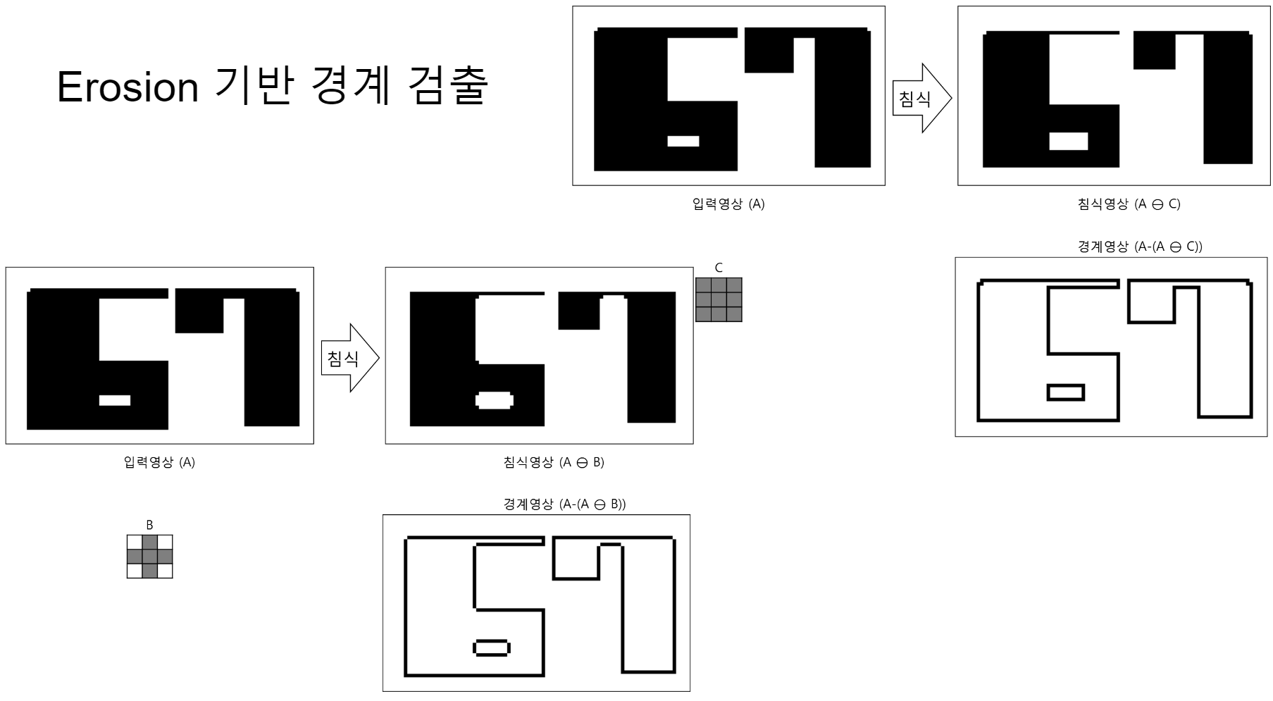
위 image에서는 어두운 부분이 255(or 1)에 해당하고, 흰색이 0에 해당함.

Morphological OP.기반 Boundary Detection의 장점.¶

참고 : Gradient

영상에서 pixel value의 변화율.

영상의 특성 중에서 edge를 판단하기 위한 중요한 요소.

Edge의 경우, gradient가 매우 큼 : pixel value가 갑자기 커지거나 작아짐.

즉, gradient가 큰 경우 edge로 판단할 수 있음.

Differentiation(미분) based method

Gradient나 Laplacian 연산을 이용함.
“이상적 영상(ideal)”에서 매우 잘 동작함.
미분의 특성상 일종의 High pass filter로 Noise도 같이 증폭시키는 단점을 가짐.
일반적으로 low-pass filter(e.g. Gaussian Filter)를 이용하여 noise를 제거하고 나서 미분을 수행.
- 이 경우, LPF로 인한 blurring으로 edge 정보가 일부 손실될 수 있음..
또한, 미분 수행 방향 에 영향을 받음.

Morphological Edge detection

Edge의 방향성에 영향을 받지 않음.
Dilation - Erosion = Edge
or (Ojbect - Erosion )

Other Morphological Operations¶

erosion, dilation, opening, closing 들이 대표적이나,
이들 외에도 많이 사용되는 operations는 다음과 같음.

Tophat¶

💡 Original - Opening

주변에 비해 밝은(높은) intensity를 가지는 부분들이 강조됨.

다음 코드는 tophat의 사용법을 보여준다.

kernel = np.ones((9,9),np.uint8)

opening = cv2.morphologyEx(out, cv2.MORPH_OPEN, kernel)
tophat = cv2.morphologyEx(img, cv2.MORPH_TOPHAT, kernel)

plt.figure(figsize=(10,5))
plt.subplot('131')
plt.imshow(img,cmap='gray'), plt.axis('off')
plt.subplot('132')
plt.imshow(opening,cmap='gray'), plt.axis('off')
plt.subplot('133')
plt.imshow(tophat,cmap='gray'), plt.axis('off')

결과는 다음과 같음.

tophat연산을 쉽게 이해하기 위한 예제임.
tophat의 효과를 보여주는 예제 이미지는 tophat과 blackhat을 비교한 예를 참고할 것.

Blackhat¶

💡 Closing - Original

주변에 비해 어두운(낮은) intensity를 가지는 부분들이 강조(binary의 경우 1로 변경)됨.

kernel = np.ones((9,9),np.uint8)

closing = cv2.morphologyEx(out, cv2.MORPH_CLOSE, kernel)
blackhat = cv2.morphologyEx(img, cv2.MORPH_BLACKHAT, kernel)

plt.figure(figsize=(10,5))
plt.subplot('131')
plt.imshow(img,cmap='gray'), plt.axis('off')
plt.subplot('132')
plt.imshow(closing,cmap='gray'), plt.axis('off')
plt.subplot('133')
plt.imshow(blackhat,cmap='gray'), plt.axis('off')

결과는 다음과 같음.

blackhat연산을 쉽게 이해하기 위한 예제임.
blackhat의 효과를 보여주는 예제 이미지는 tophat과 blackhat을 비교한 예를 참고할 것.

Tophat vs. Blackhat¶

binary image에서 tophat과 blackhat의 효과를 비교한 예는 다음과 같음.

Binary image / Left: original, Center: Tophat, Right: Blackhat — Left: original, Center: Tophat, Right: Blackhat

gray-scale image에서 tophat과 blackhat의 효과를 비교한 예는 다음과 같음.

Gray-scale image / Left: original, Center: Tophat, Right: Blackhat

다음은 위의 moon 사진에 대한 tophat과 blackhat의 효과를 profile로 보여준다.

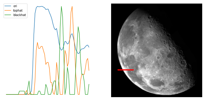
왼쪽의 달 사진의 붉은색으로 표시된 line의 profile을 보면, tophat은 주변보다 높은 값을 가진 경우 큰 값을 가지고, blackhat은 주변보다 낮은 값을 가질 경우, 큰 값을 가짐을 확인할 수 있음.

(Gray-scale에서 처리됨.)

References¶

OpenCV's tutorial
Gramman’s Morphological Transformations
Python으로 만드는 opencv프로젝트 : 6.3 모폴로지