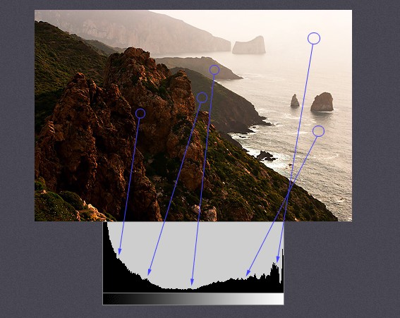
Histogram¶

Histogram은 image의 intensity (or pixel이 가지는 값)들의 분포를 보여줌.

chart로 표현하기도 하지만 내부적 데이터로 사용하기도함.

image에서 histogram으로 변환은 비가역적 변환임 (다른 image들도 같은 histogram을 가질 수 있음).

Terms¶

BINS :
- 히스토그램 그래프의 X축(intensity)의 bin의 수(histSize)를 결정 .
- 8bit gray scale 영상의 경우에는 0 ~ 255로 intensity가 표현되며, 이 경우 BINS은 최대 256 의 수를 가질 수 있음.
- 만약, BINS값이 16으로 지정할 경우, 0 ~ 15, 16 ~ 31..., 240 ~ 255와 같이 X축이 16개의 bin으로 표현이 됨.
- 이는 intensity가 0~15까지 같은 bin에서 카운팅 됨을 의미!
- OpenCV에서는 BINS를 histSize 라고 표현합니다.
channels :
- 이미지에서 histogram을 만들기 위해 사용하는 값을 의미.
- 빛의 강도(intensity)를 기준으로 histogram을 만들지, RGB값을 기준으로 만들지를 결정.
- DIMS로도 불림.
range :
- X축의 범위임 (각 pixel이 가질 수 있는 범위).
- = X축의 from ~ to.
- 원래의 pixel의 가지는 값보다 작게 지정할 경우, 해당 range의 pixel들만으로 histogram을 만들어냄.

OpenCV's Histogram¶

cv.calcHist(
    images, 
    channels, 
    mask, 
    histSize, 
    ranges
    hist, 
    accumulate
)

image : 분석대상 이미지(uint8 or float32 type). Array형태.
channels : 분석 채널(X축의 대상). 이미지가 gray-sacle이면 [0], color 이미지이면 [0,2] 형태(0 : Blue, 1: Green, 2: Red)
mask : 이미지의 분석영역. None이면 전체 영역. (0 or 255)
histSize : BINS 값. [256]
ranges : Range값. [0,256]

Example¶

#-*- coding:utf-8 -*-
import os
import cv2
import numpy as np
import random
from matplotlib import pyplot as plt

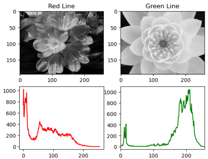
# to histogram with intensity of pixe, load image with cv2.IMREAD_GRAY 

if IN_COLAB:
    img1 = cv2.imread(os.path.join(PATH, 'flower1.jpg'), cv2.IMREAD_GRAYSCALE)
    img2 = cv2.imread(os.path.join(PATH, 'flower2.jpg'), cv2.IMREAD_GRAYSCALE)
else:
    img1 = cv2.imread('../images/flower1.jpg',0) 
    img2 = cv2.imread('../images/flower2.jpg',0)

hist1 = cv2.calcHist([img1],[0],None,[256],[0,256])
hist2 = cv2.calcHist([img2],[0],None,[256],[0,256])



#plt.style.use('dark_background')
plt.subplot(2,2,1),plt.imshow(img1,'gray'),plt.title('Red Line')
plt.subplot(2,2,2),plt.imshow(img2,'gray'),plt.title('Green Line')
plt.subplot(2,2,3),plt.plot(hist1,color='r')
plt.subplot(2,2,4),plt.plot(hist2,color='g')
plt.xlim([0,256])
plt.show()


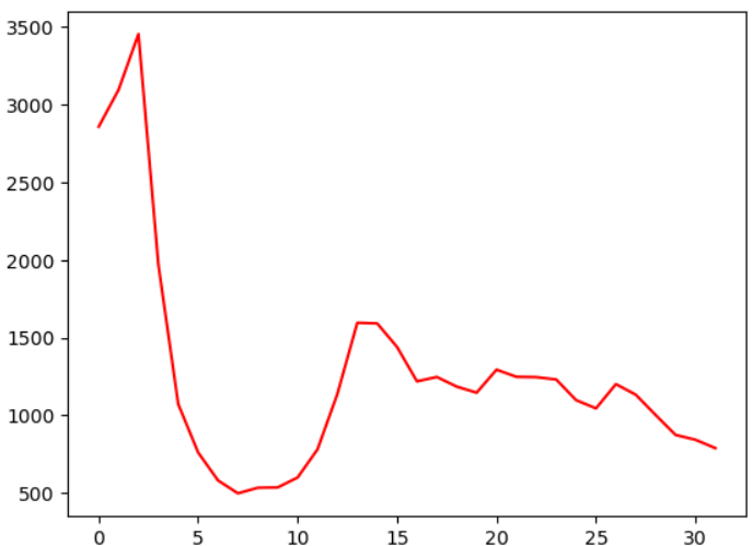
hist3 = cv2.calcHist([img1],[0],None,[32],[0,128])
print(np.shape(hist3))

plt.figure()
plt.plot(hist3,color='r')
plt.show()

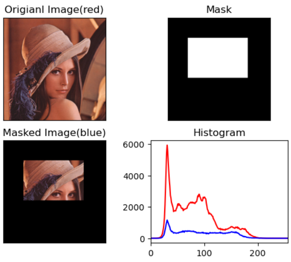
MASK사용하기.¶

#-*-coding:utf-8-*-
import cv2
import numpy as np
from matplotlib import pyplot as plt
import os


if not IN_COLAB:
    img = cv2.imread('../images/lena.png');
else:
    img = cv2.imread(os.path.join(PATH, 'lena.png'))


# mask생성
mask = np.zeros(img.shape[:2],np.uint8)
mask[100:300,100:400] = 255

# 이미지에 mask가 적용된 결과
masked_img = cv2.bitwise_and(img,img,mask=mask)

# 원본 이미지의 히스토그램 green
hist_full = cv2.calcHist([img],[1],None,[256],[0,256])

# mask를 적용한 히스트로그램 green
hist_mask = cv2.calcHist([img],[1],mask,[256],[0,256])

# bgr > rgb
#b,g,r = cv2.split(img) # divide img into b,g,r
#img = cv2.merge([r,g,b])
#b,g,r = cv2.split(masked_img)
#masked_img = cv2.merge([r,g,b])
img = img[:,:,::-1]
masked_img = masked_img[:,:,::-1]

#plt.style.use('dark_background')
plt.subplot(221),plt.imshow(img,'gray'),plt.title('Origianl Image(red)'), plt.xticks([]), plt.yticks([])
plt.subplot(222),plt.imshow(mask,'gray'),plt.title('Mask'), plt.xticks([]), plt.yticks([])
plt.subplot(223),plt.imshow(masked_img,'gray'),plt.title('Masked Image(blue)'), plt.xticks([]), plt.yticks([])

# red는 원본이미지 히스토그램, blue는 mask적용된 히스토그램
plt.subplot(224),plt.title('Histogram')
plt.plot(hist_full,color='r'),plt.plot(hist_mask,color='b')
plt.xlim([0,256])

plt.show()

Histogram Calculation in NumPy¶

hist,bin_edges = np.histogram(
    img.ravel(),
    bins = 256,
    range = [0,256],
    normed = False,
    weights = None,
    density = False
)

img : 대상 image. NumPy는 1D-array로 동작시키기 위해 ravel을 사용함. a라고 불림
bins : # of bins
range : floating point 로 주어짐. 기본은 [a.min(), a.max()]임.
normed : boolean. bin의 간격이 일정할 경우에만 True로 사용하길 권함.
weights : a와 같은 크기로 각 bin의 가중치임.
density : True이면 probability로 출력.

반환값

hist : histogram
bin_edges : bin을 나누는 edge들이라 bins+1에 대응.

2D Histograms¶

feature가 1개인 경우엔 앞서 다룬 1 dimensional histogram을 구성하지만, feature가 2개인 경우엔 2D histogram으로 처리할 수 있다.

Color space에서 HSV model을 생각해보면, V는 앞서 다룬 intensity이고, color에 해당하는 Hue와 saturation을 2D histogram으로 처리 가능하다.

(RGB를 이용하여 3D histogram도 가능은 하지만 많이 사용되지는 않는다.)

Histogram backprojection에서 H와 S를 이용하는 경우가 많기 때문에 2D histogram의 경우, Hue와 Saturation을 다루는 경우가 많다.

import numpy as np
import cv2 

img = cv2.imread('../images/2d_histogram.jpg')
assert img is not None, "file could not be read, check with os.path.exists()"

hsv = cv2.cvtColor(img,cv2.COLOR_BGR2HSV)
hist = cv2.calcHist([hsv], [0, 1], None, [180, 256], [0, 180, 0, 256])

import matplotlib.pyplot as plt

plt.subplot(1,2,1)
plt.imshow(img[...,::-1])
plt.xticks([]); plt.yticks([])
plt.subplot(1,2,2)
plt.imshow(hist, 
           interpolation='nearest', 
           cmap='jet')
plt.yticks([0,30,60,90,120,150,180])
plt.xticks([0,32,64,96,128,160,192,224,256])
# plt.colorbar()
plt.show()

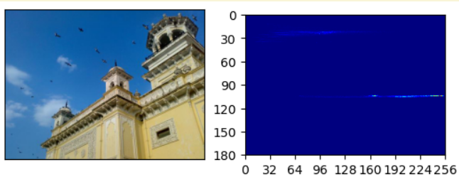
푸른 하늘에 해당하는 pixel이 많기 때문에 Hue=120 근처에서 많은 값을 보임.
건물에 해당하는 노란색도 많아서 20~30 사이에 보임.

histogram에서 잘 안보이기 때문에 V=255일 때의 HS map을 기반으로 처리한 2d histogram은 다음과 같음.

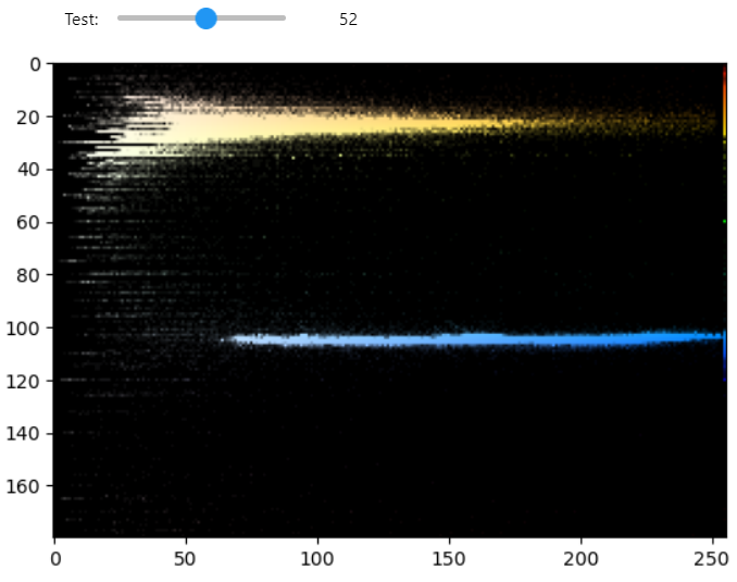
scaling의 값이 커질수록 2d histogram에서 강조가 되어 보이도록 처리함.
푸른색과 노란색 부분이 강조되어 쉽게 확인이 가능함.

Hue, Saturation은 color image의 특성을 나타내는 feature로 사용할 수 있다. (주의할 것은 다른 image라도 거의 비슷한 2d histogram을 가질 수 있다는 점임.)

pixel들의 color의 분포를 나타내는 것임.
위치적 정보가 사라지기 때문에 color들의 분포는 비슷하면 비슷한 2d histogram이 나올 수 있음.
histogram간의 유사도가 image가 같은지를 나타내는 것은 아님.

References¶

openCV's Tutorial