Geometric Transformations of Images¶

Goals¶

Learn to apply different geometric transformation to images like
- translation,
- rotation,
- affine transformation etc.
You will see these functions: cv2.getPerspectiveTransform

Transformations¶

Transformation 이란?

The function to convert(map) an specific coordinate \(\textbf{x}\) into other coordinate system \(\textbf{x}^\prime\).

Basis 를 바꾸는 것이라고 볼 수 있음.

Pre-requirements¶

다음 문서는 영상처리의 기하학적 변환의 기본이 되는 선형대수 내용이 간략히 설명됨.

2.7 Applications to Computer Graphics

1.8 Introduction to Linear Transformations

2D Geometric Image Transformations¶

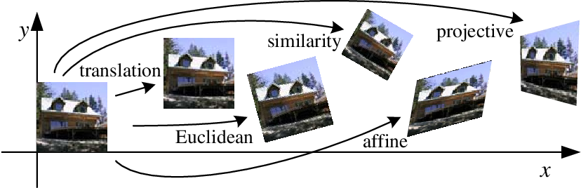
Computer Vision - Algorithms and Applications

Rigid-body(강체) transformation :¶

shape(형태), size(크기) and angle(각) are preserved.
- DoF : 3 → 2쌍 이상의 match되는 점(=4개의 값으로 갯수가 3보다 크니 충분함)이 필요.
i.e.,
- Translation,
- Rotation, and
- Identity
It is called Euclidean transformation.

\[ \begin{bmatrix} x^\prime \\ y^\prime \end{bmatrix}=\begin{bmatrix} \cos \theta & -\sin\theta \\ \sin\theta & \cos\theta \end{bmatrix}\begin{bmatrix} x \\ y \end{bmatrix}+ \begin{bmatrix} c \\ d \end{bmatrix} \]

\[\begin{bmatrix} x^\prime \\ y^\prime \\1\end{bmatrix}=\begin{bmatrix} \cos \theta & -\sin\theta &c \\ \sin\theta & \cos\theta &d \\0 & 0 & 1\end{bmatrix}\begin{bmatrix} x \\ y \\1\end{bmatrix} \]
cv2.estimateRigidTransform() 을 통해 2쌍 이상의 match되는 점들로부터 변환 matrix를 구함. (실제론 affine transform matrix를 구해줌) ← detail

Similarity transformation (or similitudes, 유사변환, 닮은변환) :¶

Rigid-body transformation + (Isotropic) Scaling
- DoF : 4 (회전각, x,y축의 translation, scaling factor)
- 2쌍 이상의 match되는 점이 있어야 파라메터 구할 수 있음.
angle is preserved but
size can be changed. (확대/축소 때문에)
i.e.,
- (Isotropic) Scaling
cv2.estimateRigidTransform() 을 통해 2쌍 이상의 match되는 점들로부터 변환 matrix를 구함. (실제론 affine transform matrix를 구해줌) ← detail

참고 : Linear transformation :¶

Function to mapping on the vector space.
It specifies
- homogeniety and
- additivity.
i.e.,
- Scaling (isotropic scaling 포함),
- Shear,
- Reflection, and
- Rotation about the origin.

Translation(이동)은 Homogeniety(동차성)을 만족하지 못함 → linear transformation이 아님. ← Homogeneous coordinate사용시 linearity를 가지게 되어 matrix곱만으로 처리 가능해짐.

Affine transformation :¶

Linear transformation + Translation.
- DoF : 6
- 3쌍의 match되는 점들이 있어야 standard matrix를 결정할 수 있음.← OpenCv에서는 \(2 \times 3\) matrix로 처리됨.
- \(\begin{bmatrix} x^\prime \\ y^\prime \\1\end{bmatrix}=\begin{bmatrix} a & b &e \\ c & d &f\\0 & 0 & 1\end{bmatrix}\begin{bmatrix} x \\ y \\1\end{bmatrix}\)
Function between affine spaces which preserves points, straight lines and planes.
선들의 평행성이 보장된다. → 임의의 평면이 임의의 평면 으로 평행성을 보존 하면서 매핑됨.

참고

cv2.getAffineTransform() 을 통해 3쌍의 match되는 점을 통해 변환matrix를 구할 수 있음.
- cv2.invertAffineTransform() 를 통해 inverse matrix도 구할 수 있음.

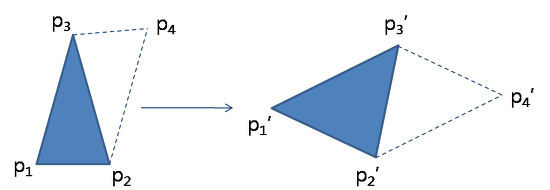
Perspective transformation (원근변환) :¶

Affine transformation w/o the property to keep parallel lines.
- 선은 변환 후에도 선으로 유지됨.
- 단, 선의 평행성은 유지가 보장되지 않음.
- 임의의 평면이 임의의 평면으로 평행성을 보존하지 않고 매핑됨.
3D 공간의 입체적인 물체를 평면에 투영하는데 사용되며 원근감이 표현됨.
- DoF : 8 (\(3\times 3\) matrix이나 homogeneous coordinate에서 마지막 component가 1로 고정이나 다름이 없기 때문에, matrix의 3행 3열의 entry가 1이라는 constant value을 가지게 되어 9-1로 8 DoF를 가짐.)
Perspective projection, Projective transformation, Homograpy 라고도 불림.
cv2.getPerspectiveTransform() 를 통해 4쌍의 match되는 점 으로부터 변환행렬 구해줌.
cv2.findHomography()는 4쌍 이상의 match되는 점들 부터 변환행렬을 구해줌(approximate method로 , fitting, RANSAC, LMedS중 선택가능)

Homography를 직관적으로 이해하기 위한 한 좋은 방법¶

2D 평면에서 임의의 사각형을 임의의 사각형으로 매핑시킬 수 있는 변환이 homography 라고 생각할 수 있음.
어떤 planer surface 촬영대상이 서로 다른 위치의 카메라로 촬영되어 image A, image B로 투영된 경우, 이 A와 B사이의 점들의 위치 관계를 homography로 표현가능함.
평면물체의 2D 이미지 변환관계를 설명함.
Projective transformation과 homography는 같은 말임.

Geometric Transformation in the OpenCV¶

OpenCV provides two geometric transformation functions,

cv2.warpAffine and
cv2.warpPerspective,

with which you can have all kinds of geometric transformations.

Note: Warping Transformation
- 굴곡 변환
- 비선형적 기하학적 연산

Affine Transformation vs. Perspective Transformation¶

Untitled

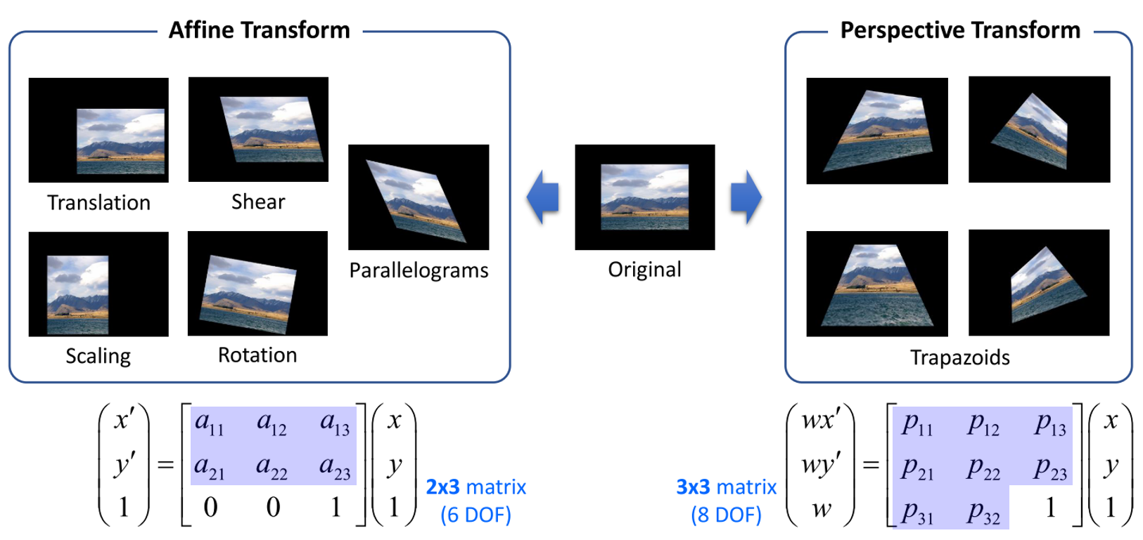
cv2.warpAffine takes

a \(2\times3\) transformation matrix (6DOFs)

while cv2.warpPerspective takes

a \(3\times3\) transformation matrix (8DOFs) as input.

Untitled

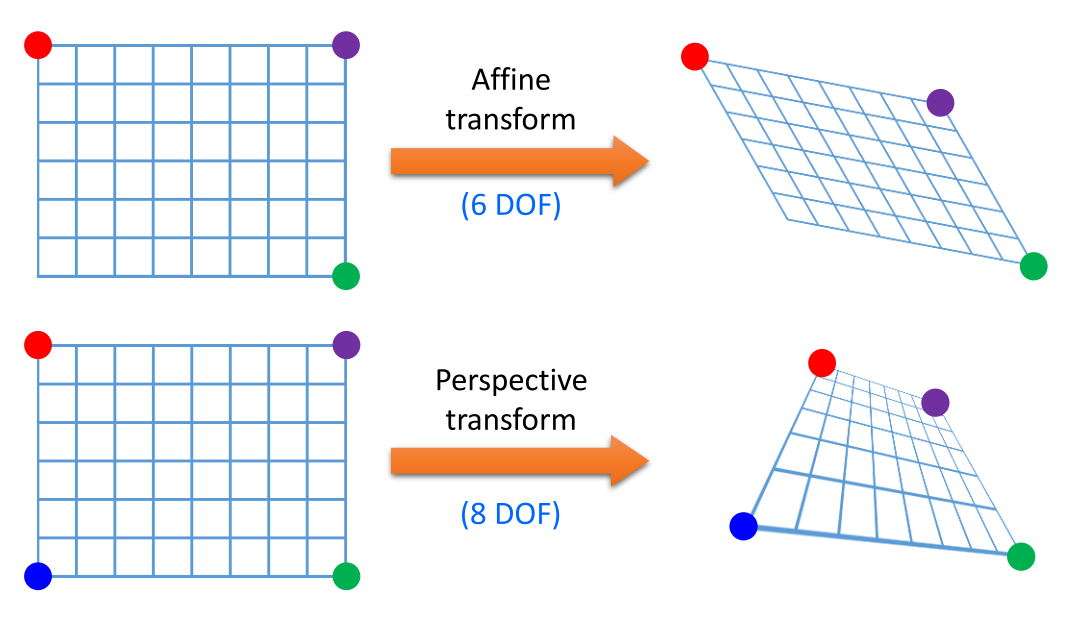
Affine Transformation에서 6개의 파라미터를 알기 위해서는 6개의 연립 방정식이 필요.
- 1개의 (x, y)에 대한 homogeneous 행렬에서 DOF에 관한 2개의 식을 구할 수 있기 때문에 3개 점의 6개 식을 이용하면 6개의 DOF를 구할 수 있음.
- 이는 위 그림과 같이 Affine Transformation이 평행사변형 형태를 유지하는 변환이기 때문에 3개의 점을 지정하면 자동적으로 하나의 점이 고정이 되어 3개의 점을 통해 변환 행렬을 구할 수 있는 것과 같은 의미임.
- 3개의 점의 변환 전 좌표와 변환 후 좌표를 알아야 Affine 변환 행렬을 구할 수 있음.
이와 동일한 관점에서 Perspective Transformation은 8개의 DOF를 구하기 위하여 4개의 점을 사용하여 구할 수 있음.
- 이는 위 그림과 같이 Perspective Transformation에서는 4개의 꼭지점이 자유롭게 변환된 상태로 이미지를 변환할 수 있어야 하기 때문에 4개의 점의 변환 전 좌표와 변환 후 좌표를 알아야 Perspective 변환 행렬을 구할 수 있음.

Translation¶

Translation is the shifting of object’s location.

If you know the shift in \((x,y)\)-direction, let it be \((t_x,t_y)\), you can create the transformation matrix \(\textbf{M}\) as follows:

\[ M = \begin{bmatrix} 1 & 0 & t_x \\ 0 & 1 & t_y \end{bmatrix} \]

You can

make it into a Numpy array of type np.float32 and
pass it into cv2.warpAffine() function.

See below example for a shift of (150,50):

python code

from skimage import data
from skimage import img_as_ubyte,img_as_float
import cv2
import numpy as np
import matplotlib.pyplot as plt

cat = data.chelsea() # take the test image of cat!
img = cv2.cvtColor(cat, cv2.COLOR_RGB2GRAY)
# img = cv2.imread('cat_cv.tif',0)

rows,cols = img.shape

M = np.float32([[1,0,150],
                [0,1,50]])

dst = cv2.warpAffine(img,M,(cols,rows))

# cv2.imshow('img',dst)
# cv2.waitKey(0)
# cv2.destroyAllWindows()
plt.figure(figsize=(12,12))
plt.subplot(121); plt.imshow(img, cmap='gray'), plt.axis('off')
plt.subplot(122); plt.imshow(dst, cmap='gray'), plt.axis('off')
plt.show()

Result

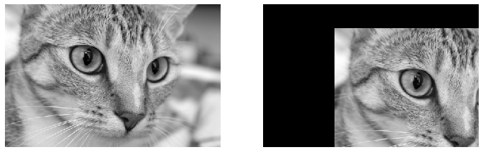
Rotation¶

Rotation of an image for an angle \(\theta\) can also be done using wrapAffine() —only the transformation matrix changes.

The transformation matrix for the rotation is as follows:

\[ M = \begin{bmatrix} \cos\theta & -\sin\theta \\ \sin\theta & \cos\theta \end{bmatrix} \]

꼬마 가 신 신고

But OpenCV provides scaled rotation with adjustable center of rotation so that you can rotate at any location you prefer.

Modified transformation matrix is given by

\[\begin{bmatrix} \alpha & \beta & (1- \alpha ) \cdot \text{center.x} - \beta \cdot \text{center.y} \\ -\beta & \alpha & \beta \cdot \text{center.x} + (1- \alpha ) \cdot \text{center.y} \end{bmatrix}\]

where:

\[ \begin{array}{l} \alpha = \text{scale} \cdot \cos \theta , \\ \beta = \text{scale}\cdot \sin \theta \end{array} \]

To find this transformation matrix, OpenCV provides a function, cv2.getRotationMatrix2D. It takes

the center for rotation (←pixel),
angle of rotation (←degree), and
isotropic scaling factor as input.
Ref. API for getRotationMatrix2D

OpenCV: Geometric Image Transformations

Check below example which rotates the image by 30 degree with respect to center without any scaling.

python code

from skimage import data
from skimage import img_as_ubyte,img_as_float
import cv2
import numpy as np
import matplotlib.pyplot as plt

cat = data.chelsea() # take the test image of cat!
img = cv2.cvtColor(cat, cv2.COLOR_RGB2GRAY)
#img = cv2.imread('cat_cv.tif',0)

rows,cols = img.shape # there is no channel

#------------------------------------
# getRotationMatrix2D
# the rotation center is given by Tupple.
# (center.x cneter.y), rotation degree, scale
M = cv2.getRotationMatrix2D((cols/2,rows/2),30,1)
print(M)

dst = cv2.warpAffine(img,M,(cols,rows))

# cv2.imshow('img',dst)
# cv2.waitKey(0)
# cv2.destroyAllWindows()

plt.figure(figsize=(12,12))
plt.subplot(121); plt.imshow(img, cmap='gray'), plt.axis('off')
plt.subplot(122); plt.imshow(dst, cmap='gray'), plt.axis('off')
plt.show()

result

[[  0.8660254    0.5        -44.78872855]
 [ -0.5          0.8660254  132.84618943]]

Untitled

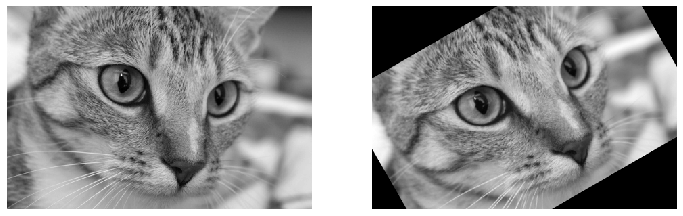
Scaling¶

Scaling is just resizing of the image.

OpenCV comes with a function cv2.resize() for this purpose.

cv2.resize(img, dsize, fx, fy, interpolation)

img : source image
dsize : desired size (specified manually), tuple (width,height)
fx : scale factor along the horizontal axis
fy : scale factor along the vertical axis
interpolation : the method of interpolation

The size of the image can be specified manually, or you can specify the scaling factor.

Different interpolation methods are used.

Preferable interpolation methods are cv2.INTER_AREA for shrinking and
cv2.INTER_CUBIC (slow) & cv2.INTER_LINEAR for zooming.

By default, interpolation method used is cv2.INTER_LINEAR for all resizing purposes.

Various interpolation algorithms are provided by OpenCv as follows;

cv2.INTER_AREA
- It is preferred for shrinking the image size.
cv2.INTER_LINEAR
- default algorithm.
- It is commonly used for zooming.
cv2.INTER_CUBIC
- It is used for zooming with a better quality but slow.
cv2.INTER_NEAREST
- Very fast but quality is not good.

You can resize an input image either of above methods:

python code

from skimage import data
from skimage import img_as_ubyte,img_as_float
import cv2
import numpy as np
import matplotlib.pyplot as plt

#img = cv2.imread('cat_cv.tif')

height, width = img.shape[:2]
print("original dimension : ({}, {}, {})".format(height,width,channel))

#-------------------
zoomed_cat = cv2.resize(img,None,fx=2, fy=2, interpolation = cv2.INTER_CUBIC)
#OR
zoomed_cat = cv2.resize(img,(2*width, 2*height), interpolation = cv2.INTER_CUBIC)
#-------------------

print("modified dimension :",zoomed_cat.shape)
cv2.imshow('zoomed_cat',zoomed_cat)
# cv2_imshow(zoomed_cat)

zoomed_cat_NN = cv2.resize(img, (2*width,2*height), interpolation = cv2.INTER_NEAREST)
cv2.imshow('zoomed_cat_NN',zoomed_cat_NN)
#cv2_imshow(zoomed_cat_NN)

cv2.waitKey(0)
cv2.destroyAllWindows()

result

original dimension : (300, 451, 3)
modified dimension : (600, 902)

Review : Cropping¶

In OpenCv, cropping is provided by using the slicing of python.

Slicing an array is just taking the array values within particular index range.

python code

import matplotlib.pyplot as plt

zoomed_cat = cv2.cvtColor(zoomed_cat,cv2.COLOR_RGB2BGR)
zoomed_cat_NN = cv2.cvtColor(zoomed_cat_NN,cv2.COLOR_RGB2BGR)

cropped_img0 = zoomed_cat[150:300,250:450]
#cv2_imshow(cropped_img0)
cropped_img1 = zoomed_cat_NN[150:300,250:450]
#cv2_imshow(cropped_img1)

plt.figure(figsize=(12,12))
plt.subplot(121); plt.imshow(cropped_img0) # expects distored color
plt.subplot(122); plt.imshow(cropped_img1) # expects true color
plt.show()

#--------------------------------------
# be careful to modify the cropped img.
tmp = cropped_img0.copy()
cropped_img0[:]=0

#cv2_imshow(zoomed_cat)
#cv2_imshow(tmp)
plt.imshow(zoomed_cat)
plt.show()
plt.imshow(tmp)
plt.show()

zoomed_cat[150:300,250:450]=tmp
#cv2_imshow(zoomed_cat)
plt.imshow(zoomed_cat)
plt.show()

result

Reflection (Flip) Transformation (대칭변환)¶

Untitled

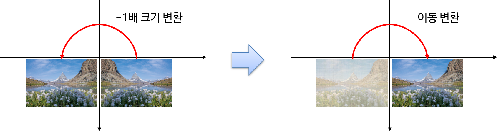
Reflection + Translation = flip
Linear Transformation : Reflections

cv2.flip(src, flipMode, dst = None) -> dst

src : input image
flipMode : +1 (좌우), 0 (상하), -1 (원점)
dst : output image

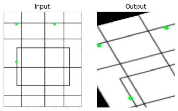
Affine Transformation¶

In affine transformation, all parallel lines in the original image will still be parallel in the output image.

To find the transformation matrix, we need three points from input image and their corresponding locations in output image.

Then cv2.getAffineTransform will create a \(2\times3\) matrix which is to be passed to cv2.warpAffine.

Check below example, and also look at the points I selected (which are marked in Green color):

python code

import cv2
import matplotlib.pyplot as plt

img = cv2.imread('images/drawing.png')
rows,cols,ch = img.shape

pts1 = np.float32([[38,38],[145,38],[38,145]])   
pts2 = np.float32([[10,100],[200,50],[100,250]])

M = cv2.getAffineTransform(pts1,pts2)

dst = cv2.warpAffine(img,M,(cols,rows))

plt.subplot(121),plt.imshow(img),plt.title('Input'),plt.axis('off')
plt.subplot(122),plt.imshow(dst),plt.title('Output'),plt.axis('off')
plt.show()

result

The example for the Affine Transformation¶

OpenCv의 mouse callback function을 이용한 예제임.

python code

import cv2
import numpy as np

points = []

# 왼쪽 상단, 오른쪽 상단, 왼쪽 하단, 오른쪽 하단 순으로 클릭하시오.

# mouse callback function
def draw_circle(event,x,y,flags,param):
    if event == cv2.EVENT_LBUTTONDBLCLK:
        global points
        cv2.circle(img,(x,y),10,(255,0,0),-1)
        print(x,y)
        points.append([x,y])


# Create a black image, a window and bind the function to window
img = cv2.imread('images/drawing.png')
rows,cols,ch = img.shape
cv2.namedWindow('image')
cv2.setMouseCallback('image',draw_circle)

while(1):
    cv2.imshow('image',img)
    if cv2.waitKey(20) & 0xFF == 27: # enter ESC
        break
    if len(points) == 3:
        pts1 = np.float32(points)
        pts2 = np.float32([[10,100],[200,50],[100,250]])
        M = cv2.getAffineTransform(pts1,pts2)        
        dst = cv2.warpAffine(img,M,(cols,rows))
        cv2.imshow('after',dst)

cv2.destroyAllWindows()

for the details : Affine Transform

Perspective Transformation¶

For perspective transformation, you need a \(3\times3\) transformation matrix.

\[ \begin{bmatrix} w\hat{x} \\ w\hat{y} \\ w \end{bmatrix}= \begin{bmatrix} a & b & c \\ d & e & f \\ g & h & 1 \end{bmatrix} \begin{bmatrix} x \\ y \\ 1 \end{bmatrix} \]

Straight lines will remain straight even after the transformation.

Perspective(원근법) 변환은 선의 성질만 유지( 직선 은 변환 후에도 직선 )
단, 선의 평행성은 유지가 되지 않음

To find Perspective Transformation Matrix, we need 4 points on the input image and corresponding points on the output image.

Among these 4 points, 3 of them should not be colinear.

Then transformation matrix can be found by the function cv2.getPerspectiveTransform.

8 variables can be obtained by following matrix equation.
8 variables = 8 Degree of Freedom (8DoF)

\[ \begin{bmatrix} \hat{x}_1 \\ \hat{y}_1 \\ \hat{x}_2 \\ \hat{y}_2 \\ \hat{x}_3 \\ \hat{y}_3 \\ \hat{x}_4 \\ \hat{y}_4 \end{bmatrix} = \begin{bmatrix} x_1 & y_1 & 1 & 0 & 0 & 0 & -x_1\hat{x}_1 & -\hat{x}_1y_1 \\ 0 & 0 & 0 & x_1 & y_1 & 1 & -x_1\hat{y}_1 & -y_1\hat{y}_1 \\ x_2 & y_2 & 1 & 0 & 0 & 0 & -x_2\hat{x}_2 & -\hat{x}_2y_2 \\ 0 & 0 & 0 & x_2 & y_2 & 1 & -x_2\hat{y}_2 & -y_2\hat{y}_2 \\ x_3 & y_3 & 1 & 0 & 0 & 0 & -x_3\hat{x}_3 & -\hat{x}_3y_3 \\ 0 & 0 & 0 & x_3 & y_3 & 1 & -x_3\hat{y}_3 & -y_3\hat{y}_3 \\ x_4 & y_4 & 1 & 0 & 0 & 0 & -x_4\hat{x}_4 & -\hat{x}_4y_4 \\ 0 & 0 & 0 & x_4 & y_4 & 1 & -x_4\hat{y}_4 & -y_4\hat{y}_4 \end{bmatrix} \begin{bmatrix} a \\ b \\ c \\ d \\ e \\ f \\ g \\ h \end{bmatrix} \]

Then apply cv2.warpPerspective with this \(3\times3\) transformation matrix.

See the code below:

python code

import cv2
import numpy as np
from matplotlib import pyplot as plt

img = cv2.imread('images/Railroad-Tracks-Perspective.jpg')
# [x,y] 좌표점을 4x2의 행렬로 작성
# 좌표점은 좌상->좌하->우상->우하
pts1 = np.float32([[504,1003],[243,1525],[1000,1000],[1280,1685]])

# 좌표의 이동점
pts2 = np.float32([[10,10],[10,1000],[1000,10],[1000,1000]])

# pts1의 좌표에 표시. perspective 변환 후 이동 점 확인.
cv2.circle(img, (504,1003), 20, (255,0,0),-1)
cv2.circle(img, (243,1524), 20, (0,255,0),-1)
cv2.circle(img, (1000,1000), 20, (0,0,255),-1)
cv2.circle(img, (1280,1685), 20, (0,0,0),-1)

M = cv2.getPerspectiveTransform(pts1, pts2)
print(type(M))
print(M)

dst = cv2.warpPerspective(img, M, (1100,1100))

plt.subplot(121),plt.imshow(img),plt.title('image')
plt.subplot(122),plt.imshow(dst),plt.title('Perspective')
plt.show()

result

<class 'numpy.ndarray'>
[[-2.02153837e+00 -1.02691611e+00  2.04001743e+03]
 [-2.24880859e-02 -3.30149532e+00  3.31389904e+03]
 [-2.62496544e-04 -1.74594051e-03  1.00000000e+00]]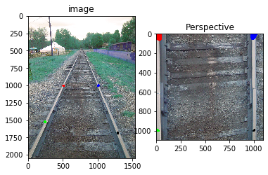

Untitled

python code 2

img = cv2.imread('images/sudokusmall.png')
rows,cols,ch = img.shape

pts1 = np.float32([[62,69],[392,54],[31,404],[413,410]])
pts2 = np.float32([[0,0],[300,0],[0,300],[300,300]])

M = cv2.getPerspectiveTransform(pts1,pts2)

dst = cv2.warpPerspective(img,M,(300,300))

plt.subplot(121),plt.imshow(img),plt.title('Input')
plt.xticks([]);plt.yticks([])
plt.subplot(122),plt.imshow(dst),plt.title('Output')
plt.xticks([]);plt.yticks([])
plt.show()

result 2

The example for the Perspective Transformation¶

OpenCv의 mouse callback function을 이용한 예제임.

import cv2
import numpy as np

points = []

# 왼쪽 상단, 오른쪽 상단, 왼쪽 하단, 오른쪽 하단 순으로 클릭하시오.

# mouse callback function
def draw_circle(event,x,y,flags,param):
    if event == cv2.EVENT_LBUTTONDBLCLK:
        global points
        cv2.circle(img,(x,y),10,(255,0,0),-1)
        print(x,y)
        points.append([x,y])


# Create a black image, a window and bind the function to window
img = cv2.imread('images/sudoku.jpg')
cv2.namedWindow('image')
cv2.setMouseCallback('image',draw_circle)

while(1):
    cv2.imshow('image',img)
    if cv2.waitKey(20) & 0xFF == 27: # enter ESC
        break
    if len(points) == 4:
        pts1 = np.float32(points)
        pts2 = np.float32([[0,0],[300,0],[0,300],[300,300]])
        M = cv2.getPerspectiveTransform(pts1,pts2)        
        dst = cv2.warpPerspective(img,M,(300,300))
        cv2.imshow('after',dst)

cv2.destroyAllWindows()

참고 : Rotation in 3D using OpenCV's `warpPerspective`¶

python code

from skimage import data
from skimage import img_as_ubyte,img_as_float
import cv2
import numpy as np
import matplotlib.pyplot as plt
'''
input: the image that you want rotated.
output: the Mat object to put the resulting file in.
alpha: the rotation around the x axis
beta: the rotation around the y axis
gamma: the rotation around the z axis (basically a 2D rotation)
dx: translation along the x axis
dy: translation along the y axis
dz: translation along the z axis (distance between lens and the object) (commonly use 200)
f: focal distance (distance between lens and image, a smaller number exaggerates the effect)

Author : Michael Jepson 
Original src : C++ 
Original src's URL : http://jepsonsblog.blogspot.com/2012/11/rotation-in-3d-using-opencvs.html
'''
def rotateImage(input, alpha, beta, gamma, dx, dy, dz, f):
    #alpha = (alpha - 90.)*np.pi/180.;
    #beta = (beta - 90.)*np.pi/180.;
    #gamma = (gamma - 90.)*np.pi/180.;
    alpha = (alpha)*np.pi/180.;
    beta = (beta)*np.pi/180.;
    gamma = (gamma)*np.pi/180.;


    # get width and height for ease of use in matrices
    h,w = input.shape[:2]
    print('height:',h,'width:',w)

    # Projection 2D -> 3D matrix
    A1 = np.array([
        [1,0,-w/2.],
        [0,1,-h/2.],
        [0,0,0],
        [0,0,1]])

    # Rotation matrices around the X, Y, and Z axis
    RX = np.array([
        [1,0,0,0],
        [0,np.cos(alpha),-np.sin(alpha),0],
        [0,np.sin(alpha), np.cos(alpha),0],
        [0,0,0,1]])

    RY = np.array([
        [np.cos(beta),0,-np.sin(beta),0],
        [0           ,1,            0,0],
        [np.sin(beta),0, np.cos(beta),0],
        [0,0,0,1]])

    RZ = np.array([
        [np.cos(gamma),-np.sin(gamma),0,0],        
        [np.sin(gamma), np.cos(gamma),0,0],
        [0           ,0,            1,0],
        [0,0,0,1]])

    # Composed rotation matrix with (RX, RY, RZ)
    R = np.dot(RZ,np.dot(RY,RX))
    R2 = RZ@RY@RX
    if not(np.array_equal(R2,R)):
        print(R2-R)

    # Translation matrix
    T = np.array([
        [1,0,0,dx],        
        [0,1,0,dy],
        [0,0,1,dz],
        [0,0,0,1]])

    A2 = np.array([
        [f,0,w/2.,0],        
        [0,f,h/2.,0],        
        [0,0,1,0]])

    # Final transformation matrix       
    M2 = np.dot(A2,np.dot(T,np.dot(R,A1)))
    M = A2 @ (T @ (R @ A1))
    if not(np.array_equal(M2,M)):
        print(M2-M)
    print(M)



    dst = cv2.warpPerspective(img,M,(w,h))
    return dst

cat = data.chelsea() # take the test image of cat!

img = cv2.cvtColor(cat, cv2.COLOR_RGB2GRAY)
#img = cv2.imread('cat_cv.tif',0)
h,w = img.shape[:2]

dst = rotateImage(img,0,0,0,0,0,50,100)

plt.figure(figsize=(20,10))    
plt.subplot(121),plt.imshow(img),plt.title('Input')
plt.xticks([]);plt.yticks([])
plt.subplot(122),plt.imshow(dst),plt.title('Output')
plt.xticks([]);plt.yticks([])
plt.show()

Geometric Transformations of Images¶

Goals¶

Transformations¶

Pre-requirements¶

2D Geometric Image Transformations¶

Rigid-body(강체) transformation :¶

Similarity transformation (or similitudes, 유사변환, 닮은변환) :¶

참고 : Linear transformation :¶

Affine transformation :¶

Perspective transformation (원근변환) :¶

Homography를 직관적으로 이해하기 위한 한 좋은 방법¶

Geometric Transformation in the OpenCV¶

Affine Transformation vs. Perspective Transformation¶

Translation¶

Rotation¶

Scaling¶

Review : Cropping¶

Reflection (Flip) Transformation (대칭변환)¶

Affine Transformation¶

The example for the Affine Transformation¶

Perspective Transformation¶

The example for the Perspective Transformation¶

참고 : Rotation in 3D using OpenCV's warpPerspective¶

References¶

참고 : Rotation in 3D using OpenCV's `warpPerspective`¶