High Pass Filter and Edge Detection¶

High Pass Filter¶

image의 spatial frequency domain에서 high frequency 영역을 통과시키는 필터를 가르킴.

Fourier transform을 이용하여 구현할 수도 있으나, spatial domain에서 convolution 연산을 통해서도 구현 가능함.

High Pass Filter의 특징.¶

요약하면 다음과 같다.

Edge Detection, Sharpening이 이루어짐.
단, Noise도 같이 강조됨

앞서 요약에서 말했듯이 High Pass Filter는 영상의 경계선(edge)와 boundary 등이 강조되는 것은 좋지만, 동시에 noise도 강조되는 단점을 수반한다.

영상에서 낮은 주파수 성분을 제거하여, 물체의 윤곽선이나 세부정보를 강조하는 edge를 검출
영상의 경계선이 더욱 선명해지는 sharpening 영상을 얻을 수 있지만, 오히려 잡음을 증가시켜 화질이 약화될 수 있음.

미분 등을 처리할 때 np.uint8을 사용할 경우, 모든 음수 값이 0으로 처리 되는데, 하얀색에서 검정색으로 변화하는 경우와 같이 gradient가 음수값을 가지게 되며 이를 0으로 처리하게 된다. 때문에 OpenCV Tutorial에서는 결과의 데이터 타입을 정밀도가 더 높으면서 부호값을 가지는 cv2.CV_16S, cv2.CV_32F, cv2.CV_64F로 지정한 뒤에 다시 cv2.CV_8U로 변환하는 것을 추천하고 있음.
자세한 건 다음 URL을 참고 : ddtype 설정

Edge Detection¶

High pass filter 또는 gradient filter등을 이용함.

Filter 등을 통해 image의 주요 feature 중 하나인 edge 검출 하는 것을 가르킴.
edge detection은 background와 foreground 를 분리(segmentation)하기 위해 필요한 가장 기본적 작업.
object recognization 에서도 기본이 되는 작업.
즉, image recognization, image segmentation 의 기본이 됨.

sharpening : edge를 검출해서 edge에 해당하는 pixel값을 강조

Differentiation (미분)¶

gradient 연산 을 입력영상에 적용.
디지털이기 때문에 실제론 difference(차분)연산임 : forward/backward difference

cv2.filter2D를 이용하여 쉽게 구현할 수 있음.

import cv2
import numpy as np
import matplotlib.pyplot as plt
from google.colab.patches import cv2_imshow

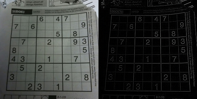
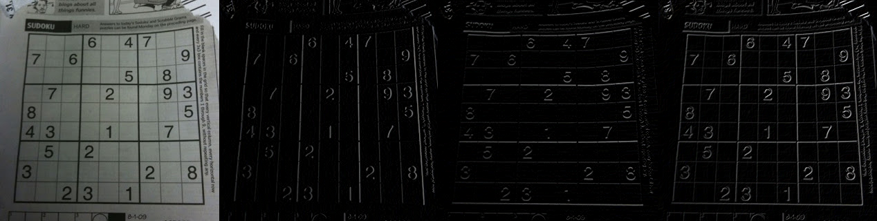
img_path = '/content/drive/My Drive/[10]Lecture/ImageProcessing/Images/sudoku.jpg'
img = cv2.imread(img_path)

#forward difference!
gx_kernel = np.array([[-1,1]])
gy_kernel = np.array([[-1],[1]])

x_edge = cv2.filter2D(img,-1,gx_kernel)
y_edge = cv2.filter2D(img,-1,gy_kernel)

results = np.hstack((img,x_edge,y_edge))
cv2_imshow(results)

cv2.filter2D의 2^nd argument는 결과의 depth정보 (desired depth, ddepth)에 해당하며, 예제와 같이 -1인 경우 1^st argument인 input image와 같은 depth를 가짐.
앞서 언급되었듯이 cv2.uint8 에서 음수를 처리 못하는 문제점으로 인해, cv2.CV_16S, cv2.CV_32F, cv2.CV_64F 등을 사용하고 이후 abs를 통해 magnitude를 구하고 cv2.CV8S등으로 casting하길 권함.

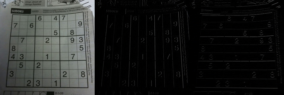
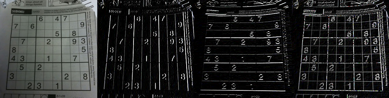
위의 코드의 결과는 다음과 같음.

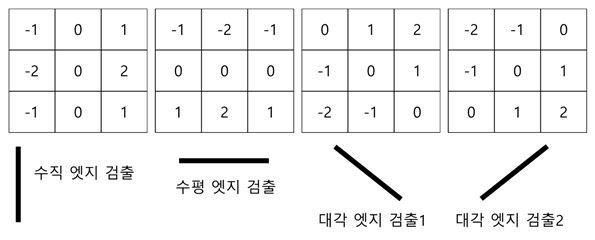
Lawrence Roberts Filter (Cross Filter)¶

1963년 로렌스 로버츠 제안.

diagonal edge를 매우 잘 검출.
noise에 약하고, 검출된 edge강도가 낮은 편.

import cv2
import numpy as np
import matplotlib.pyplot as plt
from google.colab.patches import cv2_imshow

img = cv2.imread(img_path)

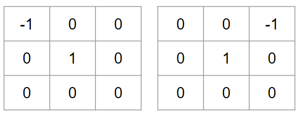
gx_kernel = np.array([[-1,0],[0,1]])
gy_kernel = np.array([[0,-1],[1,0]])

x_edge = cv2.filter2D(img,-1,gx_kernel)
y_edge = cv2.filter2D(img,-1,gy_kernel)

results = np.hstack((img,np.abs(x_edge),np.abs(y_edge),np.abs(x_edge)+np.abs(y_edge)))
#plt.imshow(results)
cv2_imshow(results)

Prewitt Filter¶

주디스 프리윗이 제안

centered difference의 digital version이라고 볼 수 있음.
It shows weak performance for diagonal edge detection.

Sobel mask의 경우와 유사한 성능에 좀더 빠른 응답시간을 보임. 단, Soble에 비해 밝기 변화에 대하여 비중이 약간 적게 준 관계로 edge가 덜 부각 됨.

import cv2
import numpy as np
import matplotlib.pyplot as plt
from google.colab.patches import cv2_imshow

img = cv2.imread(img_path)

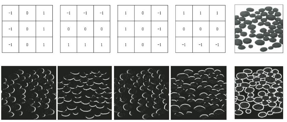
gx_kernel = np.array([
                      [-1,0,1]
])
gy_kernel = np.array([
                      [-1],[0],[1]
])

x_edge = cv2.filter2D(img,-1,gx_kernel)
y_edge = cv2.filter2D(img,-1,gy_kernel)

results = np.hstack((img,np.abs(x_edge),
                     np.abs(y_edge),
                     np.abs(x_edge)+np.abs(y_edge))
)
cv2_imshow(results)

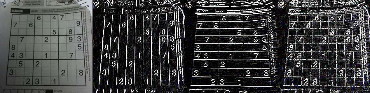
위의 코드의 결과는 다음과 같음.

Sobel Filter¶

1968년 Irwin Sobel이 제안

실무에서 널리 사용되는 1차 미분(gradient기반) 마스크 필터 : 디지털 형태의 1차미분.
1차 미분을 통한 특정방향의 Edge를 검출.
opencv에서 전용함수 제공함.
kernel이 작은 사이즈(3by3) 경우 등에서 edge의 direction(방향)에 대한 검출 정확도가 좋지 않은 단점이 있음 : Scharr filter가 이를 개선.
- Kernel이 커질수록 edge가 두꺼워지고 선명해짐.
- 단 복잡한 모양의 image나 contrast의 변화가 공간적으로 촘촘한 구간에서 일어나는 경우 위의 Kernel이 커져도 큰 효과를 보지 못함.

Sobel filter의 \(3 \times 3\) mask는 다음과 같음.

OpenCV에서 제공하는 Sobel filter의 경우, joint Gaussian smoothing과 differentiation operation을 결합하여 구현되어있으며, 다음의 function을 사용함.

cv2.Sobel(src, 
          ddepth, 
          dx, dy
          [, dst[, ksize[, scale[, delta[, borderType]]]]]
          )`

src: input
dx: x에 대한 미분 차수
dy: y에 대한 미분 차수
ksize: Sobel kernel 크기 (1,3,5,7 만 가능)

x축과 y축에 가해지는 미분 차수(degree)를 다르게 설정 (order가 아닌 degree임)할 수 있으며, kernel size (ksize)도 조절가능함.

degree 란?

\(3 \times 3\) kernel에서는 Sobel보다 뒤에 나오는 Scharr filter가 좀 더 나은 성능을 보이는 것으로 알려짐.

import cv2
import numpy as np
import matplotlib.pyplot as plt
from google.colab.patches import cv2_imshow

degree_of_diff = 1
x_edge = cv2.Sobel(img,-1,degree_of_diff,0,ksize=3)
y_edge = cv2.Sobel(img,-1,0,degree_of_diff,ksize=3)

results = np.hstack((img,np.abs(x_edge),
                     np.abs(y_edge),
                     np.abs(x_edge)+np.abs(y_edge))
)
cv2_imshow(results)

위의 코드의 결과는 다음과 같음.

Scharr Filter¶

Sobel의 단점을 개선함.

opencv에서 전용함수를 제공.
Sobel과 거의 비슷하나, ksize 설정 파라메터가 없음.

import cv2
import numpy as np
import matplotlib.pyplot as plt
from google.colab.patches import cv2_imshow

degree_of_diff = 1
x_edge = cv2.Scharr(img,-1,degree_of_diff,0)
y_edge = cv2.Scharr(img,-1,0,degree_of_diff)

results = np.hstack((img,np.abs(x_edge), # absolute value인 점을 주의할 것.
                     np.abs(y_edge),
                     np.abs(x_edge)+np.abs(y_edge))
)
cv2_imshow(results)

위의 코드의 결과는 다음과 같음.

Laplacian Filter¶

2차 미분 필터 (the 2^nd order derivative)

1차 미분 필터 (예: Sobel Filter)과 비교할 경우, 영상 내에 blob이나, 섬세(fine)한 부분을 더 잘 검출(or 강조)함.
문제는 noise도 강조한다는 점임.
매우 noise에 취약 : 사전에 Gaussian Blurring 을 취하는것이 일반적.

2차 미분은 주로 image enhancement에 사용하며 1차 미분은 feature extraction 에 사용되는 경우가 많음

noise에 민감해서 Laplacian을 단독으로 사용하기 보다 Gaussian Filter로 blurring시켜서 noise를 제거 후 Laplacian Filter를 적용하는 Laplacian of Gaussian (LoG) 를 일반적으로 사용한다.

Example :¶

\(3\times 3\) kernel로 ksize=1 인 경우의 cv2.Laplacian에서 사용됨.

\[ \begin{bmatrix}0 & 1 & 0 \\1 & -4 & 1 \\0 & 1 & 0 \end{bmatrix} \]

Taylor series로 부터 유도한 2차 미분 근사식 \(f^{\prime \prime}(x) = f(x+1) - 2f(x) + f(x-1)\) 을 2개의 독립변수로 확장시 다음과 같음.

\[ f^{\prime \prime}(x,y) = f(x-1,y) + f(x,y-1) + f(x+1,y) + f(x,y+1) - 4f(x,y) \]

이 식으로부터 위의 kernel의 weight들이 유도됨임.

OpenCV에서는 cv2.Laplacian으로 제공.

실제로 각각의 derivate는 Sobel deraivatives로 구해짐.

cv2.Laplacian(src, 
              ddepth
              [, dst
              [, ksize
              [, scale
              [, delta
              [, borderType]]]]]
              )

간단한 예제 조각 코드는 다음과 같음.

import cv2
import numpy as np
import matplotlib.pyplot as plt
from google.colab.patches import cv2_imshow

degree_of_diff = 1
edge = cv2.Laplacian(img,-1)


results = np.hstack((img,np.abs(edge)) # absolute value를 사용하는 것을 잊지 말 것.
)
cv2_imshow(results)

위의 코드의 결과는 다음과 같음.

References¶

OpenCV's Tutorial: Image Gradients