Contour Features¶

Moment¶

Image moments은 물체의 중심, 물체의 면적 등을 계산하는데 이용되는 quantity(양)임.

pixel intensity(←물리에서 force, mass등)의 정량적 크기 와 함께 분포 (어떤 기준에 대한) 를 고려한 정량적 지표.
주로 gray-scale or binary image에서 사용됨.

moment 가 가지는 뜻을 좀 더 살펴보려면 다음 URL을 참고할 것 : 물리량의 관점에서 moment란?

Spatial Moment (or raw Moment)¶

\[m_{pq} = \sum_y\sum_x x^p y^q I(x, y) \]

\(p,q\) : degree(차수)에 해당함. 0 이상의 정수가 많이 사용됨.
\(x,y\) : pixel의 x, y 좌표값
\(I(x,y)\) : x,y 위치의 pixel intensity.

(raw) moment의 값은 pixel intensity 뿐 아니라 pixel의 (절대)위치에 매우 큰 영향을 받는다.
보통 원점을 기준으로 계산된다.

Central Moment¶

앞서 본 spatial moment는 pixel의 좌표값에 영향을 크게 받기 때문에, 이미지 내에서의 절대 위치에 따라 값이 많이 바뀌게 된다.

이같은 raw moment와 달리, pixel 값의 분포로 결정되는 shape에 dependent하면서, 절대 위치에서 대해서는 가급적 독립적인 정량적 지표가 있다면, 특정 shape의 object를 검출에 유리하다.

이같은 특성으로 제안된 것이 바로 Central Moment이다.

\[\mu_{pq} = \sum_y\sum_x (x-\bar{x})^p (y-\bar{y})^q I(x, y) \]

\(\bar{x},\bar{y}\) : x, y의 mean으로 중심(image의 중심)에 해당한다.

Normalized Central Moment¶

중심 모멘트를 통해 두 이미지 상의 객체가 같은지 비교할 수 있으나, 이미지의 배율 등에 따라 central moment는 같은 object에서도 차이를 가질 수 있음. object의 전체 크기를 나누어서 좀더 robust하게 만든 것이 바로 normalized central moment임.

\[\nu_{pq}= \frac{\mu_{pq}}{\mu_{00}^{\left(1+\frac{p+q}{2}\right)}}\]

OpenCV 에서 moment구하기.¶

OpenCV에서는 cv2.moment()에 object의 contour를 넘겨줌으로서 3차까지의 moment 및 관련 수치들을 구할 수 있음.

다음 예제를 보면 moment들을 구하는 방법을 확인할 수 있다.

img = cv2.imread('star01.png', cv2.IMREAD_GRAYSCALE)
assert img is not None, "file could not be read, check with os.path.exists()"
ret,thresh = cv2.threshold(img,127,255,0)
contours,hierarchy = cv2.findContours(thresh, 
                                     cv2.RETR_LIST, 
                                     cv2.CHAIN_APPROX_SIMPLE)

cnt = contours[0]
M = cv2.moments(cnt)
print( M )

3차까지를 제공하며 Python의 dictionary로 제공한다.
다음의 키를 참고. (m : raw moment (or spatial moment, moment), mu : central moment, nu :normalized central moment)

'm00'
'm10', 'm01'
'm20', 'm11', 'm02'
'm30', 'm21', 'm12', 'm03'
'mu20', 'mu11', 'mu02'
'mu30', 'mu21', 'mu12', 'mu03'
'nu20', 'nu11', 'nu02'
'nu30', 'nu21', 'nu12', 'nu03'

Hu Moment는 일종의 global feature로 사용가능하다.

보다 자세한 건 다음 URL을 참고할 것: Hu Moement란

Hu Moment를 사용하여 shape의 similarity를 계산하는 것을 일종의 shape기반의 matching이라고도 볼 수 있음.

OpenCV에서는 cv2.matchShape()함수로 이를 제공함

Hu Moment:Match Shapes¶

object의 contour를 기반으로 object간의 shape가 유사한지 여부를 판정할 수 있음.

OpenCV는 hu-moment를 기반으로 shape의 유사도를 측정하는 cv2.matchShapes를 제공함.

ret = cv2.matchShapes(
    cnt1,
    cnt2,
    1,  # methods
    0.0 # 0.0으로 항상 입력.
    )

해당 방법에 대한 공식은 다음을 참고 : ShapeMatchMode

세번째 parameter method는 유사도 측정에 사용할 norm을 지정한다.

0 : L1을 기반.
1 : L2을 기반.
2 : L3을 기반.

즉, ret이 작을수록 비슷한 shape임을 의미함.

마지막 parameter는 세번째 parameter에 지정한 method에서 필요한 값을 넣어주기 위해 할당되었지만, 아직 제대로 지원되지 않으므로 0.0을 넣어준다.

다음 example은 아래 3개의 그림에서 A와 B의 shape의 차이, A와 C의 차이를 구함.

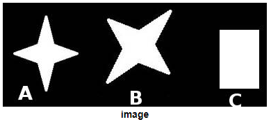
A와 B의 차이는 0.002025592564504297
A와 C의 차이는 0.3269117851861144

import cv2
import numpy as np

url = 'https://raw.githubusercontent.com/dsaint31x/OpenCV_Python_Tutorial/master/images/star.png'
image_ndarray = np.asarray(bytearray(requests.get(url).content), dtype=np.uint8)
img = cv2.imdecode(image_ndarray, cv2.IMREAD_UNCHANGED)
img = cv2.cvtColor(img, cv2.COLOR_BGRA2GRAY)
img1 = img.copy()

url = 'https://raw.githubusercontent.com/dsaint31x/OpenCV_Python_Tutorial/master/images/star2.png'
image_ndarray = np.asarray(bytearray(requests.get(url).content), dtype=np.uint8)
img = cv2.imdecode(image_ndarray, cv2.IMREAD_UNCHANGED)
img = cv2.cvtColor(img, cv2.COLOR_BGRA2GRAY)
img2 = img.copy()

url = 'https://raw.githubusercontent.com/dsaint31x/OpenCV_Python_Tutorial/master/images/rect.png'
image_ndarray = np.asarray(bytearray(requests.get(url).content), dtype=np.uint8)
img = cv2.imdecode(image_ndarray, cv2.IMREAD_UNCHANGED)
img = cv2.cvtColor(img, cv2.COLOR_BGRA2GRAY)
img3 = img.copy()

assert img1 is not None, "file could not be read, check with os.path.exists()"
assert img2 is not None, "file could not be read, check with os.path.exists()"
assert img3 is not None, "file could not be read, check with os.path.exists()"


ret, thresh  = cv2.threshold(img1, 127, 255,0)
ret, thresh2 = cv2.threshold(img2, 127, 255,0)
ret, thresh3 = cv2.threshold(img3, 127, 255,0)

contours, hierarchy = cv2.findContours(thresh,cv2.RETR_LIST,cv2.CHAIN_APPROX_SIMPLE)
cnt1 = contours[0]

contours,hierarchy = cv2.findContours(thresh2,2,1)
cnt2 = contours[0]
ret = cv2.matchShapes(cnt1,cnt2,1, 0.0)
print( ret )

contours,hierarchy = cv2.findContours(thresh3,2,1)
cnt3 = contours[0]
ret = cv2.matchShapes(cnt1,cnt3,1, 1.0)
print( ret )

Hu moment는 translation, rotation and scale에 대해 영향을 크게 받지 않는다.
자세한 건 다음을 참고할 것 :

cv2.HuMoments

Hu Moement란

Centroid¶

mass of center 라고도 자주 불림.

1차 moment로부터 구할 수 있다.

다음과 같이 1^st moment들을 0^th moment로 나누어서 구한다.

\[ c_x = \frac{m_{10}}{m_{00}}, c_y = \frac{m_{01}}{m_{00}} \]

cnt = contours[0]
M = cv2.moments(cnt)
cx = int(M['m10']/M['m00'])
cy = int(M['m01']/M['m00'])

print(cx,cy)

Contour Area¶

Contour의 넓이에 해당함.

0^th moment 에 해당하기도 한다.

cnt = contours[0]
M = cv2.moments(cnt)
print(M['m00']) # area

area = cv2.contourArea(cnt)
print(area) # area

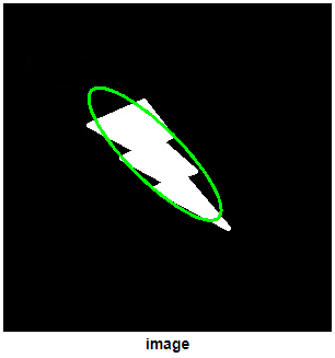
Fitting an Ellipse¶

object를 (대략) 감싸고 있는 타원을 구할 수 있음. (완전히 감싸지 않음.)

2^nd moment 를 이용하여 장축과 단축을 구하여 얻어짐.

ellipse  = cv2.fitEllipse(contours[0])
print(ellipse)
tmp0 = tmp.copy()
tmp0 = cv2.ellipse (tmp0,ellipse ,(0,255,0),2)
plt.imshow(tmp0[...,::-1])
plt.xticks([]),plt.yticks([])
plt.show()

위의 코드에서 반환되는 ellipse는 다음의 정보를 가지는 tuple임.

(
    (center_x, center_y),
    (major_axis_length, minor_axis_length),
    angle_between_x_and_major
)

(center_x, center_y) : 중점의 x,y coordinate
(major_axis_length, minor_axis_length) : ellipse의 major axis와 minor aixs의 length
angle : x-axis와 major axis의 사이각 (CW, degrees)

위의 ellipse 정보로 타원을 그리는 cv2.ellipse에 대해 자세한 건 다음 URL을 참조 : cv2.ellipse

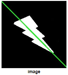
Fitting a Line¶

Object에 맞추어 놓여진 line을 구함.

역시 2^nd moment에 기반함.

rows,cols = tmp.shape[:2]
[vx,vy,x,y] = cv2.fitLine(contours[0], cv2.DIST_L2,0,0.01,0.01)
lefty = int((-x*vy/vx) + y)
righty = int(((cols-x)*vy/vx)+y)

tmp0 = tmp.copy()
cv2.line(tmp0,(cols-1,righty),(0,lefty),(0,255,0),2)
plt.imshow(tmp0[...,::-1])
plt.xticks([]),plt.yticks([])
plt.show()

Contour Perimeter¶

arc length라고도 불리는 contour의 둘레 길이. 다음의 함수로 OpenCV에서는 간단히 구할 수 있음.

perimeter = cv2.arcLength(contour[0],True)
print(perimeter)

2번째 argument는 해당 contour가 closed인지 여부를 나타냄.

Contour Approximation¶

정밀도를 지정하여, contour를 해당 정밀도 내에서 보다 간단하게 근사할 수 있음.

OpenCV에서는 이를 위해 Douglas-Peucker Algorithm의 구현물을 제공함.

대략적인 사용법은 다음과 같음.

# 전체 둘레의 5%로 오차 범위 지정 
app_rate = 0.05

# 허용가능한 정밀도의 차이 = 허용가능한 contour arclength(둘레길이)
epsilon = app_rate * cv2.arcLength(contour, True) 

# 근사 contour구하기.
approx = cv2.approxPolyDP(contour, 
                          epsilon, 
                          True)

contour : 근사치를 구하고자하는 object의 contour.
epsilon : contour arc length가 어느정도까지 줄어들 수 있는지를 나타내는 오차범위.
True : contour가 closed 인지 여부를 알려주는 argument

반환되는 approx가 근사처리된 contour임.

다음 예제를 참고.

import cv2
import numpy as np
import matplotlib.pyplot as plt
from urllib import request 

url = 'https://raw.githubusercontent.com/dsaint31x/OpenCV_Python_Tutorial/master/images/bad_rect.png'
fstr = 'bad_rect.png'
request.urlretrieve(url,fstr)
print('saved ok : bad_rect.png')

img0 = cv2.imread('./bad_rect.png')
img1 = img0.copy()

# 그레이스케일과 바이너리 스케일 변환
img_gray = cv2.cvtColor(img0, cv2.COLOR_BGR2GRAY) 
threshold, binary_img = cv2.threshold(img_gray, 127, 255, cv2.THRESH_BINARY)
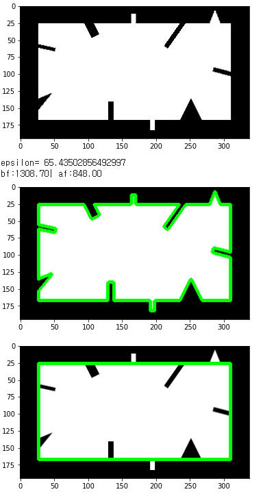
plt.imshow(binary_img,cmap='gray')
plt.show()

# 컨투어 찾기 
contours, hierarchy = cv2.findContours(binary_img.copy(), 
                                      cv2.RETR_EXTERNAL,
                                      cv2.CHAIN_APPROX_SIMPLE)
contour = contours[0]


# 전체 둘레의 5%로 오차 범위 지정 
app_rate = 0.05

#전체 contour둘레
epsilon = app_rate * cv2.arcLength(contour, True) 
print('epsilon=',epsilon)

# 근사 컨투어 계산 
# 주어진 contour(곡선 또는 다각형)을 epsilon(오차범위)에 맞춰
# contour에 속하는 점들을 줄인 approximation(근사 컨투어)를 반환
#
# param 1 : target contour
# param 2 : 오차범위
# param 3 : contour가 close인가? True : closed
approx = cv2.approxPolyDP(contour, epsilon, True)

print('bf:{:.2f}| af:{:.2f}'.format(
    cv2.arcLength(contour, True), 
    cv2.arcLength(approx, True)
    )
)

# 각각 컨투어 선 그리기 ---④
cv2.drawContours(img0, [contour], -1, (0,255,0), 3)
cv2.drawContours(img1, [approx], -1, (0,255,0), 3)

plt.figure('original contour')
plt.imshow(img0[:,:,::-1])
plt.figure('approximated contour')
plt.imshow(img1[:,:,::-1])
plt.show()

Convex Hull¶

contour에 대해서, 해당 contour를 둘러싸는 다각형을 Convex Hull이라고 부름.

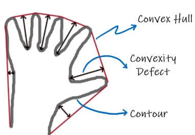
convexity defect라는 용어와 convex라는 용어의 개념을 기억할 것.

OpenCV에서는 Sklansky algorithm을 구현하여 cv2.convexHull()로 제공한다.

hull = cv2.convexHull(
    points,
    hull,
    clockwise=False,
    returnPoints=True

points : contour를 이루는 point들로 구성된 list임. 주의할 건, convexHull은 하나의 contour만을 입력으로 받는다. (복수개의 contour를 넘겨줄 수 없음)
hull : None으로 지정되는 경우가 일반적이며, 반환값이 저장된 변수명이 들어감.
clockwise : orientation으로 반환되는 convexHull을 구성하는 vertex들의 순서를 시계방향으로 할지 반시계방향으로 할지를 결정.
returnPoints : True인 경우, convexHull을 구성하는 vertex들의 좌표들로 구성된 list를 반환하고, False인 경우, 입력 argument로 들어온 points에서 convexHull에 대응하는 vertex들의 index들을 반환함.

파손이 된 부품에서 파손된 위치등을 찾는 경우에는 convexity defeat의 위치를 찾아야 하는 경우가 많다. 이 경우에는 returnPoints를 False로 넘겨주어서 contour 중에서 어떤 index의 vertex가 convexHull에 속하는지를 찾은 후, 이를 cv2.convexityDefects()에 contour와 함께 넘겨주어 찾을 수 있음.

Convexity Defects¶

cv2.convexityDefects()를 통해 찾을 수 있음.

반드시 convexHull을 구할 때, retrunPoints=False로 주고 구해야함.

hull = cv.convexHull(cnt,returnPoints = False)
defects = cv.convexityDefects(cnt,hull)

반환된 defects는 4개의 element를 가지는 vector들의 list임.

각 row에 해당하는 vector들은 다음의 정보로 구성됨.

start point : contour에서의 index에 해당함. convex hull에서의 시작점.
end point : contour에서의 index에 해당함. convex hull에서의 끝점.
farthest point : start와 end사이에 있는 convexity defect의 index (contour에서의 index)
approximate distance to farthest point.

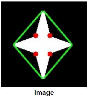
example¶

다음 예제는 convex hull을 이루는 점들은 초록색 선으로 이어서 다각형을 만들고, convexity defeat에는 붉은색의 원으로 표시를 했음.

import requests
import cv2
import numpy as np
import matplotlib.pyplot as plt

#os.makedirs('./tmp',exist_ok=True)

url = 'https://raw.githubusercontent.com/dsaint31x/OpenCV_Python_Tutorial/master/images/star.png'
image_ndarray = np.asarray(bytearray(requests.get(url).content), dtype=np.uint8)
img = cv2.imdecode(image_ndarray, cv2.IMREAD_UNCHANGED)
img = cv2.cvtColor(img, cv2.COLOR_BGRA2BGR)
tmp = img.copy()
print(img.shape)
img = cv2.cvtColor(img, cv2.COLOR_BGR2GRAY)

plt.imshow(img, cmap='gray')
plt.show()

ret,thresh = cv2.threshold(img,127,255,0)
contours,hierarchy = cv2.findContours(thresh, 
                                     cv2.RETR_LIST, 
                                     cv2.CHAIN_APPROX_SIMPLE)

hull = cv2.convexHull(contours[0],returnPoints = False)
defects = cv2.convexityDefects(contours[0],hull)

# contours[0] : (244, 1, 2)
# hull : (12, 1)
# defects : (4, 1, 4)

for i in range(defects.shape[0]):
    s,e,f,d = defects[i,0]
    start = tuple(contours[0][s][0])
    end   = tuple(contours[0][e][0])
    far   = tuple(contours[0][f][0]) # 
    cv2.line(tmp,start,end,[0,255,0],2)
    cv2.circle(tmp,far,5,[0,0,255],-1)

plt.imshow(tmp[...,::-1])
plt.xticks([]),plt.yticks([])
plt.show()

결과는 다음과 같음.

Checking Convexity¶

OpenCV는 특정 contour나 curve등이 convex인지 여부를 확인하는 function을 제공해줌.

k = cv2.isContourConvex(contours[0])
print(k)

Point Polygon Test¶

cv2.pointPolygonTest(
    conours[0], # 대상이되는 object의 contour
    (50,50), # 확인하고자 하는 point 좌표
    True # measureDist 옵션. True인 경우 signed distance를 반환. False시 [+1,-1,0]중 하나를 반환.
    )

특정 point가 object의 contour 내에 존재하는 경우에는 contour와의 거리를 양으로 반환하고, contour 밖에 있는 경우 음의 거리를 반환하여, 특정 point가 특정 object에 속하는지를 확인할 수 있음.

Bounding Rectangle¶

특정 object를 둘러싸고 있는 Bounding rectangle은 다음 그림에서 보이듯이 2가지가 존재함.

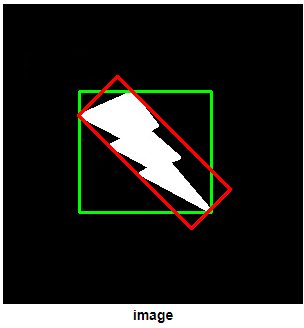
초록색의 사각형이 straight bounding rectangle이며, object의 회전 등을 고려하지 않음.
- cv2.boundingRect()를 통해 구해짐.
붉은색의 사각형은 rotated bounding rectangle이라고 불림.
- cv2.minAreaRect()를 통해 구해짐.

straight bounding rectangle¶

x,y,w,h = cv.boundingRect(contours[0])

하나의 contour를 넘겨주면 됨.

rotated bounding rectangle¶

(x,y), (w,h), angle_of_rot = cv2.minAreaRect(contours[0])

위와 같이 처리하는 것보다, 다음을 이용하는게 보다 간편함.

rect = cv2.minAreaRect(contours[0])
box = cv2.boxPoints(rect)
box = np.int0(box)
cv2.drawContours(tmp,[box],0,(0,0,255),2)

위에서 얻어진 rect를 cv2.boxPoints를 통해 4개의 vertex를 얻어낼 수 있음.

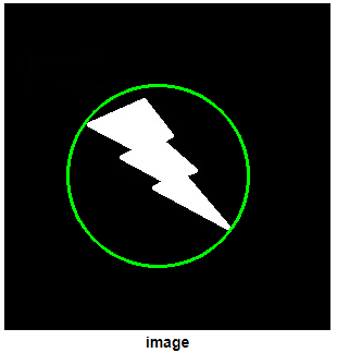
Minimum Enclosing Circle¶

object를 감싸고 있는 원을 구할 수 있음.

(x,y),radius = cv2.minEnclosingCircle(contours[0])
center = (int(x),int(y))
radius = int(radius)
tmp0 = tmp.copy()
tmp0 = cv2.circle(tmp0,center,radius,(0,255,0),2)
plt.imshow(tmp0[...,::-1])
plt.xticks([]),plt.yticks([])
plt.show()