2. Drawing Functions in OpenCV¶

다음의 ipynb 파일을 활용할 것.

관련 ipynb파일

2-0. Goal¶

OpenCV 를 이용하여 선,원, 사각형, 글자 등을 그리는 방법을 배운다.

실질적으로 다음의 함수들을 사용하는 법을 배운다. :

cv2.line()
cv2.circle()
cv2.rectangle()
cv2.ellipse()
cv2.putText()

2-1. Common Parameters¶

우리가 다루게 될 function들에서 자주 등장하는 common argument는 다음과 같음.

img: 실제로 우리가 그리는 도형이나 글자가 그려질 image 객체.
numpy의 ndarray 객체임.
color: 도형이나 글자의 색.
컬러 이미지의 경우 BGR로 지정되고, gray-scale인 경우는 scalar값으로 처리 가능함.
tuple로 Blue, Green, Red 의 값을 [0,255] 로 기재하는 형태로 주는 것을 권함.
thickness: 도형 등의 line(선)의 두께. 만일 -1이 넘겨질 경우 채워줘서 그려짐 (또는 cv2.FILLED 로 지정).
default thickness = 1
lineType: 선의 형태,
cv2.LINE_4(4-connected),
cv2.LINE_8(8-connected),
cv2.LINE_AA(anti-aliased line) 중에서 선택.
default line type = cv2.LINE_8.

2-2. Drawing Line¶

cv2.line을 이용하여 라인을 그린다.

시작점,
끝점,
선의 두께,
색 등을 argument로 넘겨줌.

다음 예제를 보자.

import numpy as np
import cv2

# Create a black image
img = np.zeros((512,512,3), np.uint8)

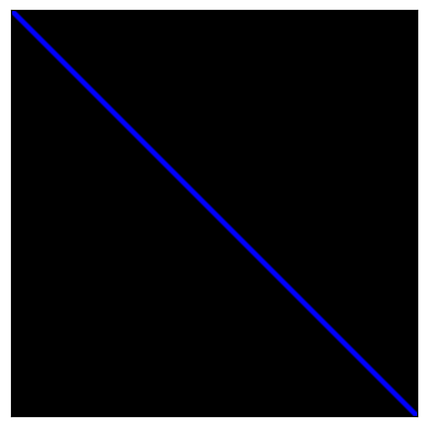
# Draw a diagonal blue line with thickness of 5 px
img = cv2.line(img,
               (0,0),       # pnt0
               (511,511),   # pnt1
               (255,0,0),   # color
               5            # thickness
               )

다음을 통해 line(선)을 확인 가능함.

from matplotlib import pyplot as plt

imt2 = img[:,:,::-1].copy() //BGR to RGB
plt.imshow(img2)
plt.xticks([]); plt.yticks([]) # to hide tick values on X and Y axis
plt.show()

다음은 결과 이미지임.

2-3. Drawing Rectangle¶

사각형을 그리기 위해서,

top-left corner 와
bottom-right corner of rectangle 를

arguments 로 넘겨줌.

다음 예제를 참고하라.

import numpy as np
import cv2

# Create a black image
img = np.zeros((512,512,3), np.uint8)

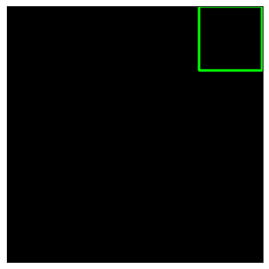
img = cv2.rectangle(img,       # 그려지는 대상. 
                    (384,0),   # top-left
                    (510,128), # bottom-right
                    (0,255,0), # color, BGR
                    3          # thickness
                    )

다음 조각코드로 오른쪽 상단에 사각형을 확인할 수 있음.

from matplotlib import pyplot as plt

img2 = img[:,:,::-1].copy() //BGR to RGB for matplotlib
plt.imshow(img2)
plt.xticks([]); plt.yticks([]) # to hide tick values on X and Y axis
plt.show()

다음은 결과 이미지임.

2-4. Drawing Circle¶

원을 그리는 경우,

center의 좌표와
radius를

argument로 넘겨줌.

다음 예제를 보자.

import numpy as np
import cv2

# Create a black image
img = np.zeros((512,512,3), np.uint8)

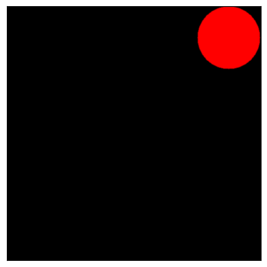
img = cv2.circle(img,         # target image
                 (447,63),    # center
                 63,          # radius
                 (0,0,255),   # color
                 cv2.FILLED,  # thickness : -1 means cv2.FILLED
                 )
print(f'{cv2.FILLED:d}')

다음 조각코드로 오른쪽 상단에 red circle(원)을 확인할 수 있음.

from matplotlib import pyplot as plt

img2 = img[:,:,::-1].copy() //BGR to RGB for matplotlib
plt.imshow(img2)
plt.xticks([]); plt.yticks([]) # to hide tick values on X and Y axis
plt.show()

다음 결과를 확인할 것.

2-5. Drawing Ellipse¶

타원(ellipse)을 그리기 위한 arguments는 다음과 같음.

타원의 중점 좌표 : (x,y).
타원의 first axis과 second axis의 길이 : (first axis length, second axis length).
- 아래 그림에서는 AXES.WIDTH, AXES.HEIGHT 로 기재됨.
- first axis를 major axis (장축) 으로도 지칭하는 경우도 있는데 엄밀히는 조금 틀린 명칭임
- major axis 는 장축을 의미하지만, openCV에서 first axis는 second axis보다 길이가 짧을 수 있음 .
- first axis 는 ellipse의 회전 각도 angle이 0 인 경우 x-axis 가 되는 축임.
- second axis 는 ellipse의 회전 각도 angle이 0 인 경우 y-axis 가 되는 축임.
타원의 회전 각도 : angle (clockwise direction and degrees).
- first axis와 x-axis의 각도.
- 아래 그림 참조할 것.
타원의 arc (호)를 그리기 위한 시작각과 끝각을 argument로 받음 :startAngle and endAngle
- clockwise direction
- degree 로 지정됨.
- major axis(or first axis)가 x-axis 를 기준으로 회전한 이후의 시작 각도가 더해지는 방식.

For more details, check the documentation of cv2.ellipse().

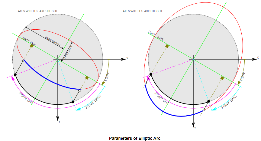
first axis(=AXES.WIDTH)와 second axis(=AXES.HEIGHT)의 길이는 타원의 중심에서 타원의 각 축과의 거리임(원의 반지름에 해당)
위 그림에서는 AXES.WIDTH , AXES.HEIGHT 로 기재됨 (왼쪽 그림에서 AXES.WIDTH의 길이 확인할 것.).

주의할 점은 ellipse관련 각도는 arc-angles이고 circular angle이 아님.

The angles used in ellipse function is not our circular angles.

Starting angle and ending angle are measured in arc-angles from an ellipse, not from a circle.

The phenomena is visualized in paragraph (59) of http://mathworld.wolfram.com/Ellipse.html .

visit this discussion : (https://answers.opencv.org/question/14541/angles-in-ellipse-function/)

다음 예제를 살펴보자.

img = np.zeros((512,512,3), np.uint8)
img = cv2.ellipse(img,
                  (256,256), # center
                  (100,200), # first axis length, second axis length : radius
                  20,        # rotation angle (CW)
                  70,        # start angle (CW)
                  80,        # end angle (CW)
                  255,       # color (gray-scale or [255,0,0]과 같음.) 
                  -1         # filled 
                  )

arc를 그리지 않는 경우는 다음의 같이 사용하기도 함.

img = np.zeros((512,512,3), np.uint8)
img = cv2.ellipse(img,
                  [
                    (256,256), # center
                    (200,400), # bounding box width, bounding box height
                    20,       # rotation angle (CW)
                  ],
                  [0,0,255],   # color  
                  -1           # filled (-1) or thickness (0 초과 양수) 
                  )

이 경우, 2^nd argument가 ellipse에 대한 정보를 다 가지고 있음.
이 전의 경우와 달리, 타원을 둘러싸는 bounding box의 넓이와 높이로 주어짐: (즉, 지름에 해당한다고 생각할 것.)
이 전과 같아지려며 2배를 해 줘야 함.
cv2.fitEllipse 로 contour를 둘러싸는 타원을 계산할 때의 반환값이 바로 2^nd argument로 들어가는 정보임.

ref. : fitEllipse

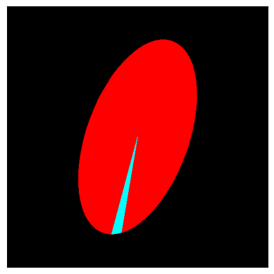
다음 조각코드 수행시 중앙에 타원이 보인다. (arc가 일부만 되도록 한 부분 주의할 것.)

from matplotlib import pyplot as plt

img2 = img[:,:,::-1].copy() //BGR to RGB for matplotlib
plt.imshow(img2)
plt.xticks([]); plt.yticks([]) # to hide tick values on X and Y axis
plt.show()

위의 2코드를 동시에 그린 결과는 다음과 같음: (arc를 그리는 예를 수행한 결과임)

2-6. Drawing Polygon¶

다각형을 그리는 방법은 다음과 같음.

우선 각 vertex의 좌표들의 ndarray를 생성. (rows x 2)
해당 ndarray를 rows x 1 x 2 로 reshape를 시킨다. rows는 vertex들의 숫자에 해당.
해당 ndarray는 int32 를 dtype로 가짐.

사실, 위의 내용은 tutorial의 내용이나, 실제로 reshape를 하지 않고도 동작함.

다음의 예제를 참고.

pts = np.array([[10,5],[120,330],[320,120],[150,100]], 
               np.int32) # x,y
print(pts.shape)

# pts = pts.reshape((-1,1,2)) #openCV 튜토리얼에서 권하는 구현이나 생략해도 그려짐.
print(pts.shape)

img = cv2.polylines(img,        # target image
                    [pts],      # vertices
                    True,       # isClosed (닫혔는지여부)
                    (0,255,255),# color
                    1,          # thickness
                    )

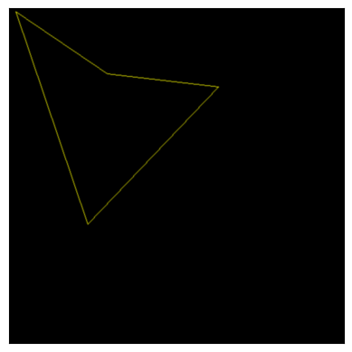
다음의 조각코드를 수행하여 확인 가능함.
4개의 점이 연결된 다각형이 그려짐.

from matplotlib import pyplot as plt

img2 = img[:,:,::-1].copy() //BGR to RGB for matplotlib
plt.imshow(img2)
plt.xticks([]); plt.yticks([]) # to hide tick values on X and Y axis
plt.show()

결과 이미지는 다음과 같음.

2-6-0. Note0 : `cv2.polylines`¶

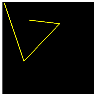
cv2.polylines의 세번째 argument 가 False이면
닫힌 다각형이 아닌 "끝점과 시작점이 연결이 안 된 상태" 로 그려짐을 확인할 수 있음.

test_img = np.zeros_like(img)
test_img = cv2.polylines(test_img,[pts],False,(0,255,255),4)

img2 = test_img[:,:,::-1].copy()
plt.imshow(img2,interpolation='bicubic'
           )
plt.xticks([]); plt.yticks([]) # to hide tick values on X and Y axis
plt.show()

결과 이미지는 다음과 같음

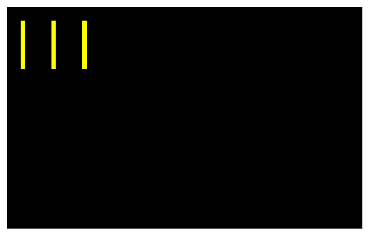
2-6-1. Note1 : `cv2.polylines` 의 용도¶

cv2.polylines() 은 실제로 여러 개의 라인을 그리는데 사용 된다.

여러 선에 해당하는 list를 argument로 넘기면 해당 선들이 그려진다.
cv2.line() 을 여러번 호출하는 것보다 처리 효율이 좋다.

다음 코드를 통해 사용 방법을 익혀보자.

pts0 = np.array(
    [[3,3],[3,13]]
    ,np.int32).reshape(-1,1,2)
pts1 = np.array(
    [[10,3],[10,13]]
    , np.int32).reshape(-1,1,2)
pts2 = np.array(
    [[17,3],[17,13]]
    , np.int32).reshape(-1,1,2)
print(np.array([pts0,pts1,pts2]).shape) # (3, 2, 1, 2)

test_img = np.zeros((50,80,3), np.uint8)
test_img = cv2.polylines(test_img,[pts0,pts1,pts2],False,(0,255,255))

img2 = test_img[:,:,::-2].copy()
plt.imshow(img2, interpolation='bicubic')
plt.xticks([]); plt.yticks([]) # to hide tick values on X and Y axis
plt.show()

결과 이미지는 다음과 같음.

2-7. 꽉 찬 다각형 그리기.¶

보통 다음 두 가지 functions를 사용한다.

cv2.fillConvexPoly(img,points,color): points에 저장된 좌표로 이루어진 볼록다각형을 color로 채운다.
fillPoly보다 빠르지만, 오목한 경우 다르게 칠해진다.
cv2.fillPoly(img,contours,color): 하나 이상의 다각형 을 color 색상으로 칠한다.
contours=[points_of_contour0, ...]

일반적으로 contour 등을 구한 경우, 경계좌표 들로 라벨링을 해야할 때 위 2개의 함수가 이용되는데
fillConvexPoly는 하나의 볼록 다각형을 가정 하기 때문에
오목한 경우 제대로 그려지지 않는 경우가 많다.

가급적 fillPoly 또는 cv2.drawContours를 사용하는 것이 좋다.

참고 : cv2.drawContours

fillPoly 와 cv2.drawContours는 여러 개 의 꽉 찬 다각형을 처리하도록 구현됨.
list 로 여러 다각형을 한 번에 넘김.
fillConvexPoly는 하나의 꽉찬 볼록 다각형을 그리는 것으로 구현됨.
하나의 다각형만을 argument로 넘김 (pnt 로 구성된 list)

다음 예제를 참고할 것..

import cv2
import numpy as np
import matplotlib.pyplot as plt

src = np.zeros((300, 300, 3), dtype=np.uint8)

img = src.copy()
points = np.array(
    [[100, 50], [200, 100], 
     [200, 140], [50, 250], [130,100], 
     [270, 120], [220, 50],
     [100, 60]
     ])
points_a = np.array([[5,5], [10,10], [5,30]])

img = cv2.fillPoly(img, [points,points_a], color=(0, 255, 0))
img2 = img[:,:,::-1].copy()
plt.imshow(img2)

img = src.copy()
img = cv2.fillConvexPoly(img, points, color=(0, 255, 0))
img2 = img[:,:,::-1].copy()
plt.figure()
plt.imshow(img2)

cv2.fillPoly는 여러 개의 다각형을 그리므로 넘겨지는 것이 다각형들의 꼭지점을 가진 list들의 list임 : [points,points_a].
cv2.fillConvexPoly는 하나의 다각형에 대한 꼭지점들의 list가 넘겨진다.
이 예제에서는 오목형 다각형 이라 cv2.fillConvexPoly는 제대로 그려지지 않음을 확인할 수 있음.

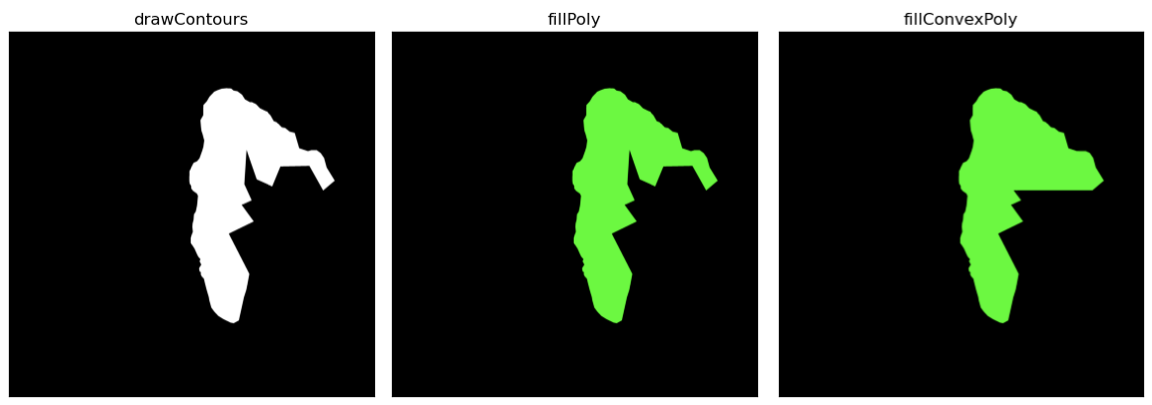
다음 코드는 cv2.fillConvexPoly의 사용법을 같이 보여준다.

src = np.zeros((3000, 3000, 3), dtype=np.uint8)
img = src.copy()

points = np.array([
   [2148,  687],[2120,  658],[2100,  650],[2062,  631],
   [2028,  596],[1994,  580],[1978,  580],[1938,  557],[1914,  519],
   [1877,  491],[1845,  485],[1825,  468],[1785,  466],[1747,  470],
   [1716,  481],[1687,  494],[1648,  535],[1626,  573],[1598,  604],
   [1597,  640],[1597,  687],[1574,  727],[1578,  782],[1582,  816],
   [1593,  849],[1597,  866],[1605,  895],[1598,  947],[1589,  978],
   [1566, 1043],[1546, 1067],[1518, 1080],[1506, 1104],[1482, 1148],
   [1481, 1227],[1484, 1251],[1498, 1271],[1498, 1289],[1514, 1310],
   [1544, 1331],[1554, 1350],[1546, 1433],[1536, 1481],[1521, 1504],
   [1518, 1548],[1510, 1579],[1508, 1606],[1512, 1647],[1493, 1698],
   [1493, 1739],[1504, 1752],[1525, 1784],[1548, 1836],[1557, 1853],
   [1574, 1872],[1567, 1889],[1581, 1917],[1563, 1946],[1566, 1971],
   [1577, 1978],[1577, 1998],[1585, 2014],[1602, 2032],[1621, 2112],
   [1631, 2147],[1642, 2184],[1647, 2213],[1663, 2271],[1688, 2305],
   [1720, 2339],[1763, 2366],[1821, 2394],[1846, 2399],[1888, 2376],
   [1930, 2185],[1946, 2136],[1951, 2117],[1974, 1993],[1805, 1662],
   [2010, 1562],[1910, 1425],[1993, 1387],[1933, 1255],[1951,  970],
   [2035, 1215],[2163, 1273],[2230, 1109],[2468, 1104],[2581, 1306],
   [2675, 1226],[2609, 1118],[2588, 1040],[2561, 1000],[2528,  976],
   [2484,  976],[2456,  984],[2384,  960],[2347,  834],[2306,  824],
   [2269,  794],[2242,  789],[2198,  744],[2176,  736],[2173,  731]])

print(points.shape)

# points가 리스트에 다시 담겨서 argument넘겨짐. 주의.
img = cv2.drawContours(img, [points], -1, (255,255,255), thickness=-1)
plt.figure()
plt.title('drawContours')
plt.xticks([]);plt.yticks([])
img2 = img[:,:,::-1].copy()
plt.imshow(img2)

img = src.copy()
cv2.fillPoly(img, [points], color=(0, 255, 0)) # points 가 list에 담겨서 
plt.figure()
plt.title('fillPoly')
plt.xticks([]);plt.yticks([])
img2 = img[:,:,::-1].copy()
plt.imshow(img2)

img = src.copy()
cv2.fillConvexPoly(img, points, color=(0, 255, 0)) # points가 직접 arguments로.
plt.figure()
plt.title('fillConvexPoly')
plt.xticks([]);plt.yticks([])
img2 = img[:,:,::-1].copy()
plt.imshow(img2)

결과는 다음과 같음

2-8. Adding Text to Images:¶

우선 한글 출력이 안 된다.. --;;
한글은 matplotlib 를 추천.
cv2.putText는 Unicode 지원이 안되는게 최대 단점임.

image에 글자를 추가하려면 다음과 같이 처리한다.

우선 글자에 해당하는 문자열 데이터 생성.
bottom-left corner로 해당 text 가 놓일 위치를 지정.
Font type 을 지정. (Check cv2.putText() docs for supported fonts)
Font Scale 을 지정. (specifies the size of font)
color, thickness, lineType 등을 지정.

For better look, lineType = cv2.LINE_AA is recommended.